Updates to dataRetrieval 2026
Introduction
In this ~90 minute introduction, the goal is:
Introduce new
dataRetrievalfunctionsThe intended audience is someone:
Seasoned
dataRetrievaluserAND/OR intermediate R user
Familiar with USGS water data
New to dataRetrieval? Introduction to dataRetrieval
Why are we here?
NWIS servers are shutting down
That means all
readNWISfunctions will eventually stop workingTimeline is very uncertain, so we wanted to get information out on replacement functions ASAP.
New
dataRetrievalfunctions are available to replace the NWIS functionsread_waterdata_functions are the modern functionsThey use the new USGS Water Data APIs
Installation
dataRetrieval is available on the Comprehensive R Archive Network (CRAN) repository. To install dataRetrieval on your computer, open RStudio and run this line of code in the Console:
Then each time you open R, you’ll need to load the library:
Whether you are a user or developer we recommend installing dataretrieval in a virtual environment. This can be done using something like virtualenv or conda.
or
Then each time you open Python, you’ll need to load the library:
USGS Water Data OGC APIs: Current Functions
Open Geospatial Consortium (OGC), a non-profit international organization that develops and promotes open standards for geospatial information. OGC-compliant interfaces to USGS water data:
read_waterdata_monitoring_location - Monitoring location information
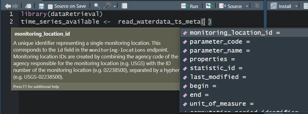
read_waterdata_ts_meta - Time series availability
read_waterdata_parameter_codes - Parameter code information
USGS Water Data OGC APIs: Current Functions (cont.)
read_waterdata_field_meta - Field measurement data availability
read_waterdata_combined_meta - Combined time series and field data availability
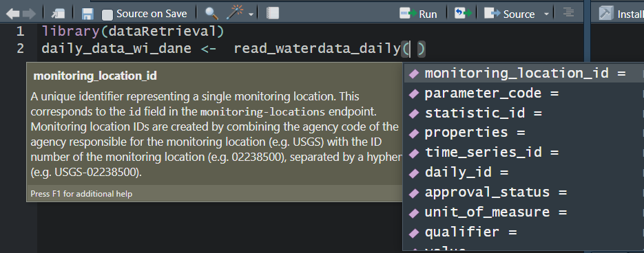
read_waterdata_daily - Daily data
read_waterdata_latest_daily - Latest daily data
USGS Water Data OGC APIs: Current Functions (cont.)
read_waterdata_continuous - Continuous data are collected via automated sensors installed at a monitoring location.
read_waterdata_latest_continuous - Latest continuous data
read_waterdata_field_measurements - Discrete hydrologic data (gage height, discharge, and readings of groundwater levels)
USGS Water Data OGC APIs: Current Functions (cont.)
read_waterdata_channel - Channel measurements
read_waterdata - Generalized function.
read_waterdata_metadata - Metadata
read_waterdata_rating - Rating Curve Data
read_waterdata_peaks - Peak Data
USGS Water Data API Token
The Water Data APIs limit how many queries a single IP address can make per hour
You can run new
dataRetrievalfunctions without a tokenYou might run into errors quickly. If you (or your IP!) have exceeded the quota, you will see:
! HTTP 429 Too Many Requests.
  • You have exceeded your rate limit. Make sure you provided your API key from https://api.waterdata.usgs.gov/signup/, then either try again later or contact us at https://waterdata.usgs.gov/questions-comments/?referrerUrl=https://api.waterdata.usgs.gov for assistance.
USGS Water Data API Token
Request a USGS Water Data API Token: https://api.waterdata.usgs.gov/signup/
Save it in a safe place (KeyPass or other password management tool)
Add it as environment variable
Restart
See next slide for a demonstration.
Water Data API Token: Example
Let’s pretend the token sent you was “abc123”
- Run in R:
- Add this line to the file that opens up:
API_USGS_PAT = "abc123"Save that file
Restart R/RStudio.
Check that it worked by running (you should see your token printed in the Console):
Note
Your .Renviorn file should never be pushed to a public repository.
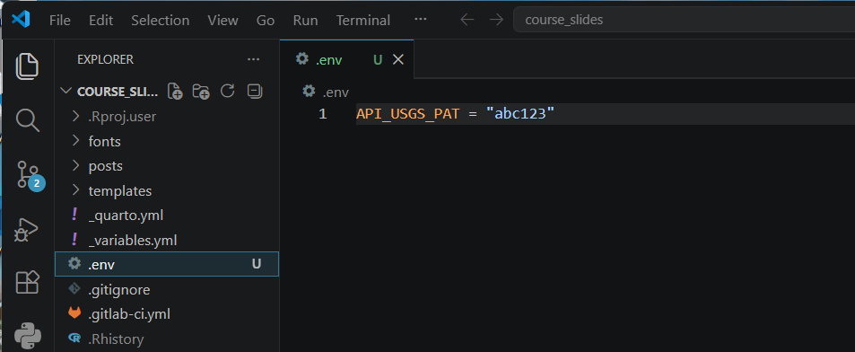
Create a file in your working directory .env
Add this line to the .env file:
API_USGS_PAT = "abc123"Restart your python session
Check that it worked by running (you should see your token printed in the Console):
Note
Make sure to add .env file to .gitignore to make sure you do not accidently push it to a public repository.
Water Data API Token: Example

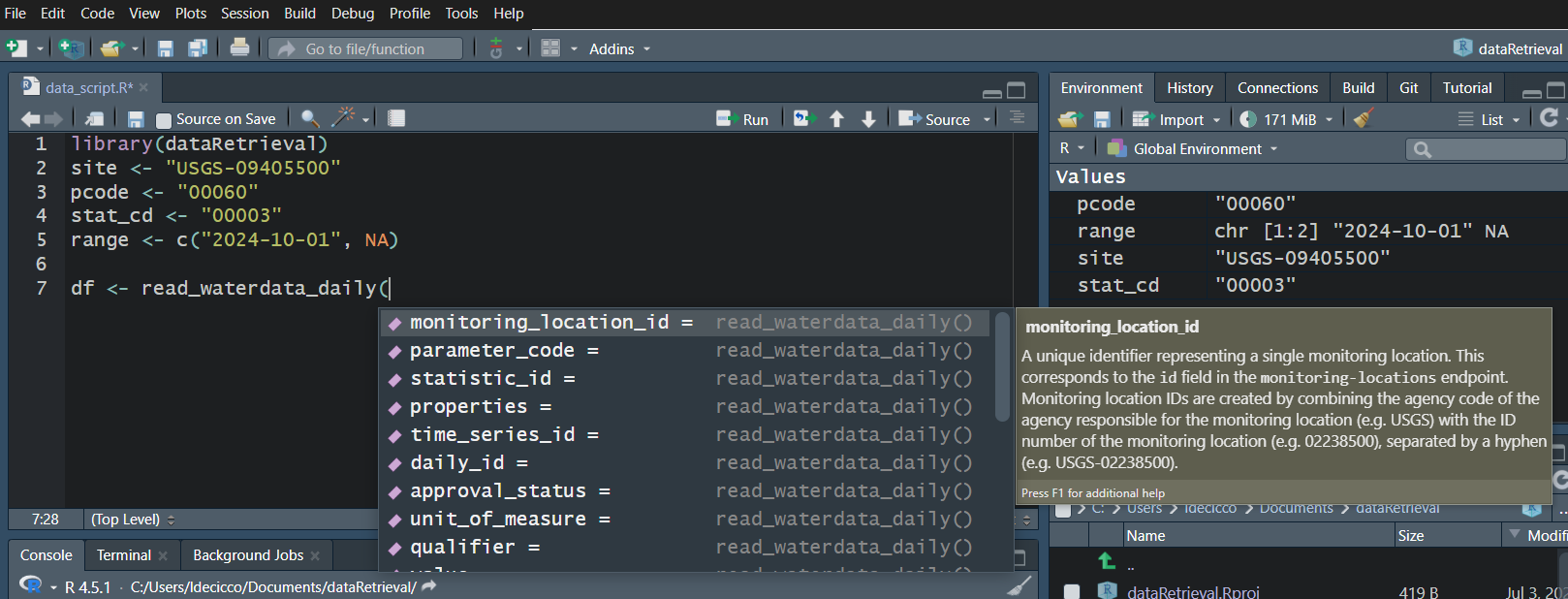
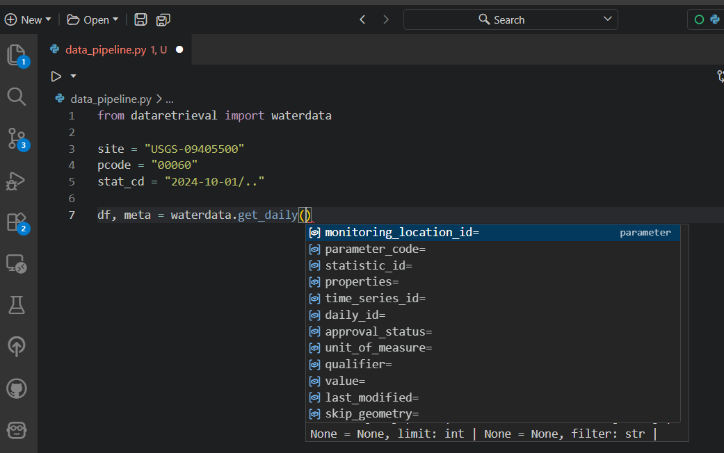
Water Data APIs: Initial Tips
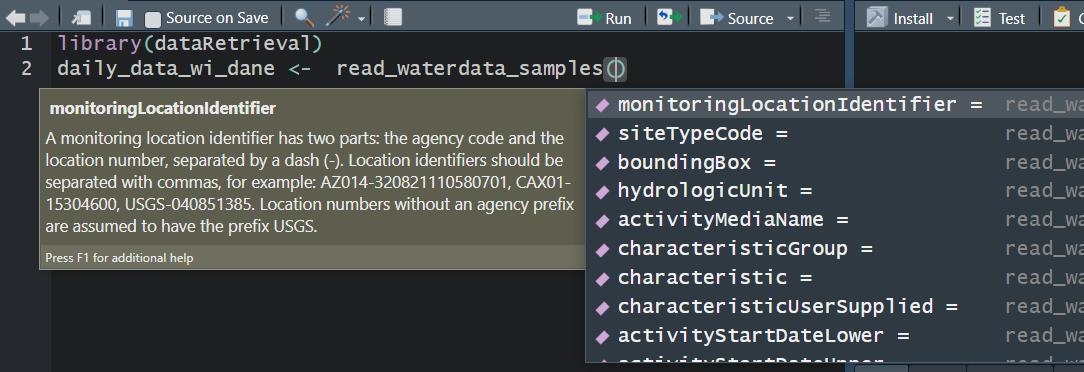
Use your “tab” key!
read_waterdata_monitoring_location
Replaces readNWISsite:
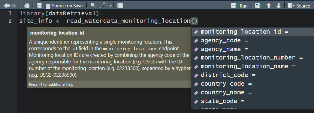
All the columns that you retrieve, you can also filter on.
You should not specify all of these parameters.
You should not specify too few of these parameters.
read_waterdata_monitoring_location
Let’s get all the monitoring locations for Dane County, Wisconsin:
Requesting:
https://api.waterdata.usgs.gov/ogcapi/v0/collections/monitoring-locations/items?f=json&lang=en-US&state_name=Wisconsin&county_name=Dane%20County&limit=50000
Remaining requests this hour:1309 read_waterdata_monitoring_location
read_waterdata_monitoring_location
Now that we’ve seen the whole data set, maybe we realize in the future we can ask for just stream sites, and we only really need a few of those columns:
Requesting:
https://api.waterdata.usgs.gov/ogcapi/v0/collections/monitoring-locations/items?f=json&lang=en-US&properties=monitoring_location_name%2Cdrainage_area&state_name=Wisconsin&county_name=Dane%20County&site_type=Stream&limit=50000
Remaining requests this hour:1309 Map It with geometry
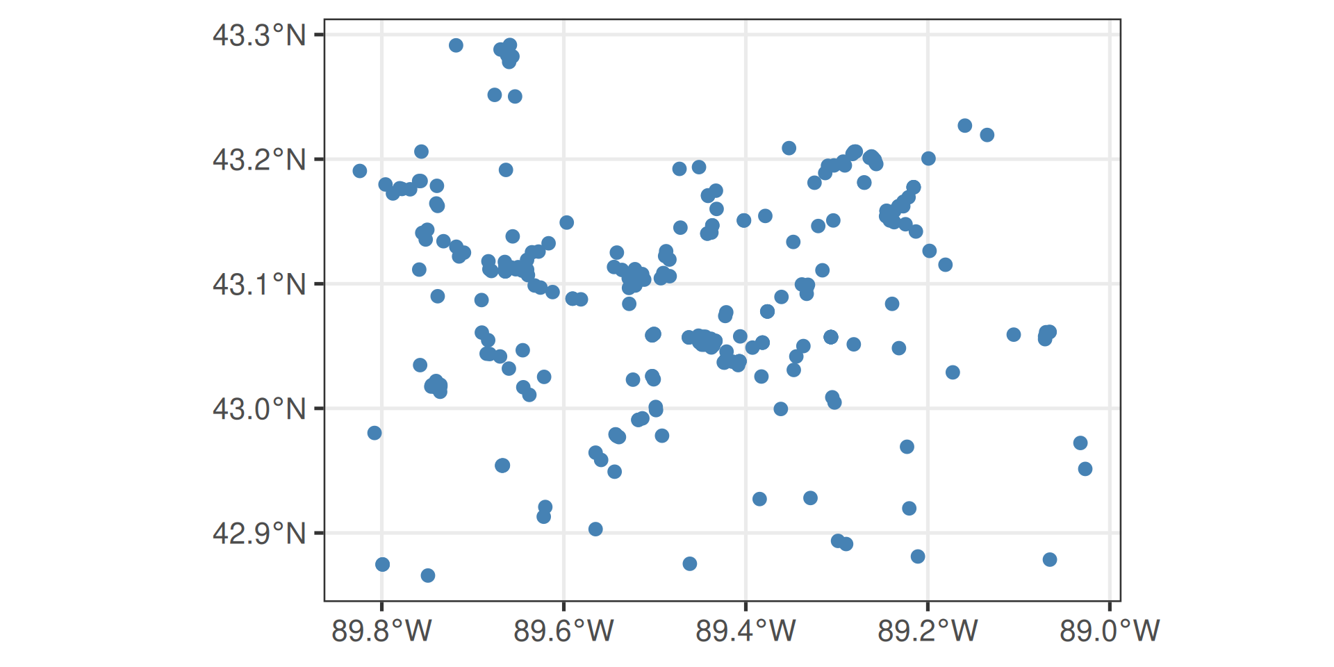
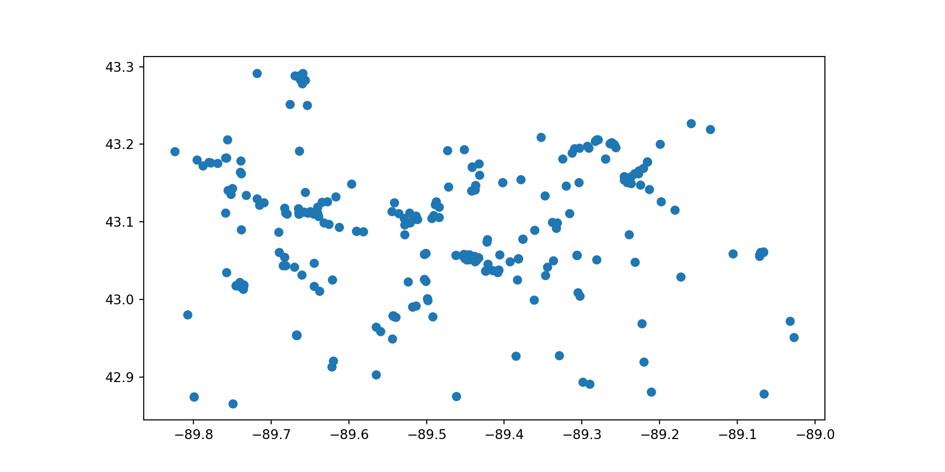
Map It: leaflet
Map It: leaflet
Removing sf
- You can post-process the “geometry” column out, or convert it to lat/lon with the
sfpackage:
- You can declare
skipGeometry=TRUEin the query to return a plain data frame with no geometry:
read_waterdata_combined_meta
Combined Time-Series Metadata. Kind of replaces whatNWISdata:
read_waterdata_combined_meta
read_waterdata_combined_meta
Let’s get all the time series in Dane County, WI with daily mean (statistic_id = “00003”) discharge (parameter code = “00060) or temperature (parameter code =”00010):
Tip
Geographic filters are limited to monitoring_location_id and bbox in “waterdata” functions other than read_waterdata_monitoring_location and read_waterdata_combined_meta.
Using sf::st_bbox() is a convenient way to take advantage of the spatial features integration.
read_waterdata_combined_meta
read_waterdata_daily
Replaces readNWISdv:
read_waterdata_daily
read_waterdata_daily
USGS Water Data APIs Notes: time input
The “time” argument has a few options:
A single date (or date-time): “2024-10-01” or “2024-10-01T23:20:50Z”
A bounded interval: c(“2024-10-01”, “2025-07-02”)
Half-bounded intervals: c(“2024-10-01”, NA)
Duration objects: “P1M” for data from the past month or “PT36H” for the last 36 hours
Here are a bunch of valid inputs:
# Ask for exact times:
time = "2025-01-01"
time = as.Date("2025-01-01")
time = "2025-01-01T23:20:50Z"
time = as.POSIXct(
  "2025-01-01T23:20:50Z",
  format = "%Y-%m-%dT%H:%M:%S",
  tz = "UTC"
)
# Ask for specific range
time = c("2024-01-01", "2025-01-01") # or Dates or POSIXs
# Asking beginning of record to specific end:
time = c(NA, "2024-01-01") # or Date or POSIX
# Asking specific beginning to end of record:
time = c("2024-01-01", NA) # or Date or POSIX
# Ask for period
time = "P1M" # past month
time = "P7D" # past 7 days
time = "PT12H" # past hours
read_waterdata_latest_continuous
Most recent observation for each time series of continuous data.
Continuous data are collected via automated sensors installed at a monitoring location. They are collected at a high frequency and often at a fixed 15-minute interval.
latest_uv_data <- read_waterdata_latest_continuous(
  monitoring_location_id = "USGS-01491000",
  parameter_code = "00060",
)

latest_dane_county <- read_waterdata_latest_continuous(
  bbox = sf::st_bbox(site_info),
  parameter_code = "00060"
)

single_ts <- read_waterdata_latest_continuous(
  time_series_id = "202345d175874d2c814648ac9bea5deb"
)read_waterdata_latest_continuous
Latest discharge observation (00060) in Dane County, WI:
Map Latest Discharge Observation: leaflet
pal <- colorNumeric("viridis", latest_dane_county$value)
leaflet_crs <- "+proj=longlat +datum=WGS84"
leaflet(
  data = latest_dane_county |>
    sf::st_transform(crs = leaflet_crs)
) |>
  addProviderTiles("CartoDB.Positron") |>
  addCircleMarkers(
    popup = paste(
      latest_dane_county$monitoring_location_id,
      "<br>",
      latest_dane_county$time,
      "<br>",
      latest_dane_county$value,
      latest_dane_county$unit_of_measure
    ),
    color = ~ pal(value),
    radius = 3,
    opacity = 1
  ) |>
  addLegend(
    pal = pal,
    position = "bottomleft",
    title = "Latest Discharge",
    values = ~value
  )
Map Latest Discharge Observation: leaflet
read_waterdata_latest_daily
Most recent observation for each time series of daily data.
Map Latest Daily Discharge: leaflet
pal <- colorNumeric("viridis", latest_dane_county_daily$value)
leaflet_crs <- "+proj=longlat +datum=WGS84"
leaflet(
  data = latest_dane_county_daily |>
    sf::st_transform(crs = leaflet_crs)
) |>
  addProviderTiles("CartoDB.Positron") |>
  addCircleMarkers(
    popup = paste(
      latest_dane_county_daily$monitoring_location_id,
      "<br>",
      latest_dane_county_daily$time,
      "<br>",
      latest_dane_county_daily$value,
      latest_dane_county_daily$unit_of_measure
    ),
    color = ~ pal(value),
    radius = 3,
    opacity = 1
  ) |>
  addLegend(
    pal = pal,
    position = "bottomleft",
    title = "Latest Discharge",
    values = ~value
  )
Map Latest Daily Discharge: leaflet
read_waterdata_continuous
Replaces readNWISuv:
Currently only allows 3 years of data to be queried at once.
More information https://water.code-pages.usgs.gov/dataRetrieval/articles/continuous_pr.html
read_waterdata
This function is totally different!
Uses CQL2 Queries: Common Query Language (CQL2)
Great examples here: https://api.waterdata.usgs.gov/docs/ogcapi/complex-queries/
read_waterdata
Wisconsin and Minnesota sites with a drainage area greater than 1000 mi^2:
read_waterdata: Map It
pal <- colorNumeric("viridis", sites_mn_wi$drainage_area)
leaflet_crs <- "+proj=longlat +datum=WGS84"
leaflet(
  data = sites_mn_wi |>
    sf::st_transform(crs = leaflet_crs)
) |>
  addProviderTiles("CartoDB.Positron") |>
  addCircleMarkers(
    popup = ~monitoring_location_name,
    color = ~ pal(drainage_area),
    radius = 3,
    opacity = 1
  ) |>
  addLegend(
    pal = pal,
    position = "bottomleft",
    title = "Drainage Area",
    values = ~drainage_area
  )
read_waterdata: Map It
read_waterdata_metadata
The function read_waterdata_metadata gives access to the metadata collections from the USGS Water Data API.
agency_codes <- read_waterdata_metadata("agency-codes")
altitude_datums <- read_waterdata_metadata("altitude-datums")
aquifer_codes <- read_waterdata_metadata("aquifer-codes")
aquifer_types <- read_waterdata_metadata("aquifer-types")
coordinate_accuracy_codes <- read_waterdata_metadata(
  "coordinate-accuracy-codes"
)
coordinate_datum_codes <- read_waterdata_metadata("coordinate-datum-codes")
coordinate_method_codes <- read_waterdata_metadata("coordinate-method-codes")
huc_codes <- read_waterdata_metadata("hydrologic-unit-codes")
national_aquifer_codes <- read_waterdata_metadata("national-aquifer-codes")
parameter_codes <- read_waterdata_metadata("parameter-codes")
reliability_codes <- read_waterdata_metadata("reliability-codes")
site_types <- read_waterdata_metadata("site-types")
statistic_codes <- read_waterdata_metadata("statistic-codes")
topographic_codes <- read_waterdata_metadata("topographic-codes")
time_zone_codes <- read_waterdata_metadata("time-zone-codes")
agency_codes, md1 = waterdata.get_reference_table("agency-codes")
altitude_datums, md2 = waterdata.get_reference_table("altitude-datums")
aquifer_codes, md3 = waterdata.get_reference_table("aquifer-codes")
aquifer_types, md4 = waterdata.get_reference_table("aquifer-types")
coordinate_accuracy_codes, md1 = waterdata.get_reference_table(
"coordinate-accuracy-codes"
)
coordinate_datum_codes, md1 = waterdata.get_reference_table("coordinate-datum-codes")
coordinate_method_codes, md1 = waterdata.get_reference_table("coordinate-method-codes")
huc_codes, md1 = waterdata.get_reference_table("hydrologic-unit-codes")
national_aquifer_codes, md1 = waterdata.get_reference_table("national-aquifer-codes")
parameter_codes, md1 = waterdata.get_reference_table("parameter-codes")
reliability_codes, md1 = waterdata.get_reference_table("reliability-codes")
site_types, md1 = waterdata.get_reference_tablea("site-types")
statistic_codes, md1 = waterdata.get_reference_table("statistic-codes")
topographic_codes, md1 = waterdata.get_reference_table("topographic-codes")
time_zone_codes, md1 = waterdata.get_reference_table("time-zone-codes")General New Features of Water Data OGC APIs
Flexible Queries
Lots of options to define your query
Do NOT define all of them
Do NOT define to few of them
Flexible Columns Returned
- Use the properties argument to ask for just the columns you want
Simple Features
- Returns a geometry column that allows seamless integration with
sf
- Returns a geometry column that allows seamless integration with
CQL query support
Lessons Learned
-
There is a character limit to how big your query can be
dataRetrievalv2.7.25 will automatically chunk up requests of long lists of monitoring_location_id.
Adding API token to CI jobs: GitLab
If you run dataRetrieval calls in a CI job, you’ll need to add an API Token to the configuration.
Go to: Settings -> CI/CD -> Variables -> Add Variable
Key should be API_USGS_PAT, value will be the token
Click on Masked and hidden
Add to your .gitlab-ci.yml file:
variables:
  API_USGS_PAT: "${API_USGS_PAT}"
Adding API token to CI jobs: GitHub
In GitHub:
Settings -> Secrets and variables -> Actions -> Secrets
Secret can be stored in Environment or Repository
If you created an Environment called “CI_config”, your CI yaml will need:
    environment: CI_config
    env:
      API_USGS_PAT: ${{ secrets.API_USGS_PAT }}
Adding API token: Posit Connect
You’ll want to add a token for any Posit Connect product (Shiny app, Quarto slides, etc.).

OR

Discrete Data
USGS switched to Aquarius Samples March 11, 2024.
On that day, the USGS data in the Water Quality Portal was frozen.
“modern USGS discrete data” = data that includes pre and post Aquarius Samples conversion.
The new function
read_waterdata_samplesgets modern USGS discrete data.- it is outside the Water Data OGC API ecosystem, so looks and feels a bit different.
Water Quality Portal (WQP) also has modern USGS discrete data, but not by default.
If you only need USGS data, use
read_waterdata_samples, if you need USGS and non-USGS, usereadWQPdata.
read_waterdata_samples
Replaces readNWISqw
USGS Samples Data Notes: Data Types and Profiles
- There are 2 arguments that dictate what kind of data is returned
- “dataType” defines what kind of data comes back
- “dataProfile” defines what columns from that type come back
Data Types and Profiles
read_waterdata_samples
That’s a LOT of columns that come back.
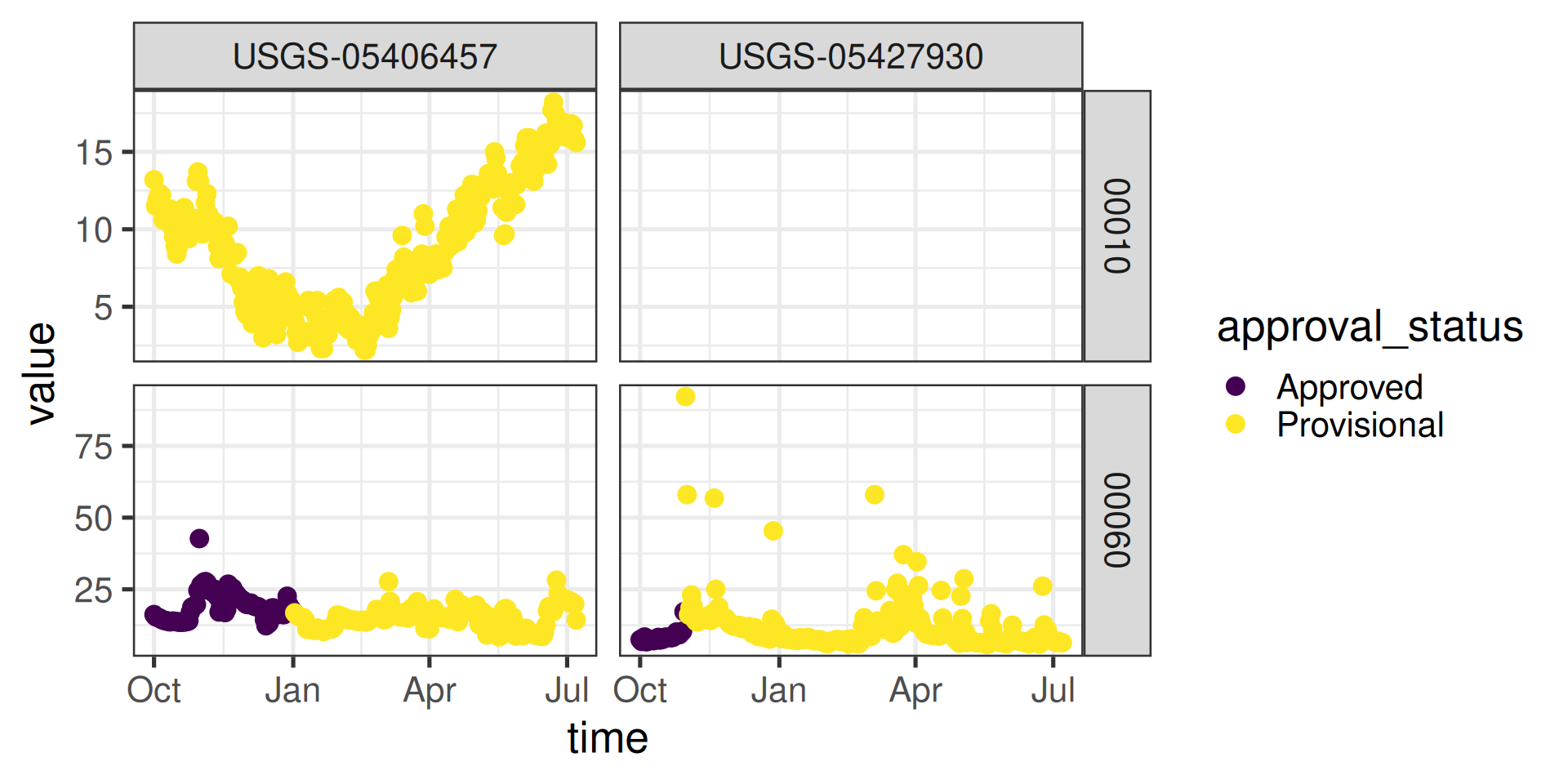
Discrete data censoring
Let’s pull just a few columns out and look at those:
library(dplyr)

qw_data_slim <- qw_data |>
  select(
    Date = Activity_StartDate,
    Result_Measure,
    DL_cond = Result_ResultDetectionCondition,
    DL_val = DetectionLimit_MeasureA,
    DL_type = DetectionLimit_TypeA
  ) |>
  mutate(
    nwis_value = if_else(DL_cond != "", DL_val, Result_Measure),
    Detected = if_else(DL_cond != "", "Not Detected", "Detected")
  ) |>
arrange(Detected)- What is
|>? It’s a pipe! It says take ‘this thing’ and put it in ‘that thing’. You’ll also see%>%in code, it is also a pipe - they are basically the same.
import numpy as np

qw_data_slim = (
    qw_data.rename(
        columns={
            "Activity_StartDate": "Date",
            "Result_ResultDetectionCondition": "DL_cond",
            "DetectionLimit_MeasureA": "DL_val",
            "DetectionLimit_TypeA": "DL_type",
        }
    )[["Date", "Result_Measure", "DL_cond", "DL_val", "DL_type"]]
    .assign(
        nwis_value=lambda x: np.where(
            x["DL_cond"].notna(), x["DL_val"], x["Result_Measure"]
        )
    )
    .assign(
        Detected=lambda x: np.where(x["DL_cond"].notna(), "Not Detected", "Detected")
    )
    .sort_values(by="Detected", ascending=False)
)
Discrete data censoring information
summarize_waterdata_samples
A summary service exists for 1 site at a time (so in this case, monitoringLocationIdentifier cannot be a vector of sites):
Water Quality Portal
If you use readWQPqw, add “legacy=FALSE” to get modern USGS data:
If you use readWQPdata, add ‘service = “ResultWQX3”’:
HELP!
There’s a lot of new information and changes being presented. There are going to be scripts that have been passed down through the years that will start breaking once the NWIS servers are decommissioned.
Check back on the documentation often: https://doi-usgs.github.io/dataRetrieval/
Peruse the “Additional Articles” - when we find common issues people have with converting their old workflows, we will try to add articles to clarify new workflows.
If you have additional questions, email comptools@usgs.gov.
Additional New Features:
More Information
- dataRetrieval repository:
- Documentation:
- Contact:
- Computational Tools Email: comptools@usgs.gov
- Bug reports can be reported here:
Any use of trade, firm, or product name is for descriptive purposes only and does not imply endorsement by the U.S. Government.