Introduction to dataRetrieval
dataRetrieval: External Documentation
dataRetrieval: External Documentation
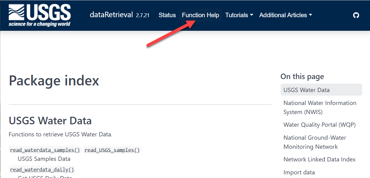
dataRetrieval: External Documentation
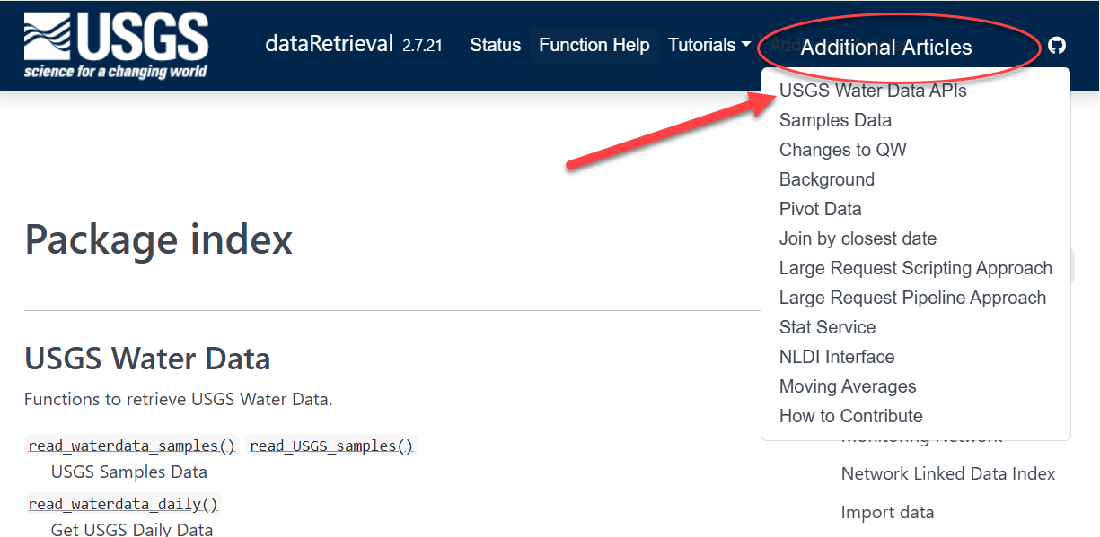
Documentation within R: function help pages
Within R, you can call help files for any dataRetrieval function:

Within Python, you can call help for any dataretrieval function:
Help on function get_daily in module dataretrieval.waterdata.time_series:

get_daily(
    monitoring_location_id: 'str | Iterable[str] | None' = None,
    parameter_code: 'str | Iterable[str] | None' = None,
    statistic_id: 'str | Iterable[str] | None' = None,
    properties: 'str | Iterable[str] | None' = None,
    time_series_id: 'str | Iterable[str] | None' = None,
    daily_id: 'str | Iterable[str] | None' = None,
    approval_status: 'str | Iterable[str] | None' = None,
    unit_of_measure: 'str | Iterable[str] | None' = None,
    qualifier: 'str | Iterable[str] | None' = None,
    value: 'str | Iterable[str] | None' = None,
    last_modified: 'str | Iterable[str] | None' = None,
    skip_geometry: 'bool | None' = None,
    time: 'str | Iterable[str] | None' = None,
    bbox: 'list[float] | None' = None,
    limit: 'int | None' = None,
    filter: 'str | None' = None,
    filter_lang: 'FILTER_LANG | None' = None,
    convert_type: 'bool' = True,
    max_rows: 'int | None' = None,
    **queryables: 'Any'
) -> 'tuple[pd.DataFrame, BaseMetadata]'
    Get daily values: one value per monitoring location, parameter, and day.

    Throughout much of the history of the USGS, the primary water data available
    was daily data collected manually at the monitoring location once each day.
    With improved availability of computer storage and automated transmission of
    data, the daily data published today are generally a statistical summary or
    metric of the continuous data collected each day, such as the daily mean,
    minimum, or maximum value. Daily data are automatically calculated from the
    continuous data of the same parameter code and are described by parameter
    code and a statistic code. These data have also been referred to as “daily
    values” or “DV”.

    Parameters
    ----------
    monitoring_location_id : string or iterable of strings, optional
        A unique identifier representing a single monitoring location,
        corresponding to the id field in the monitoring-locations endpoint. IDs
        combine the agency code of the agency responsible for the monitoring
        location (e.g. USGS) with the location's ID number (e.g. 02238500),
        separated by a hyphen (e.g. USGS-02238500).
    parameter_code : string or iterable of strings, optional
        A 5-digit code identifying the constituent measured and the units of
        measure. A complete list of parameter codes and associated groupings is
        available at https://help.waterdata.usgs.gov/codes-and-parameters/parameters.
    statistic_id : string or iterable of strings, optional
        A code corresponding to the statistic an observation represents.
        Example codes include 00001 (max), 00002 (min), and 00003 (mean).
        A complete list of codes and their descriptions can be found at
        https://help.waterdata.usgs.gov/code/stat_cd_nm_query?stat_nm_cd=%25&fmt=html.
    properties : string or iterable of strings, optional
        The columns to return from the query.
        Available options are: geometry, id, time_series_id,
        monitoring_location_id, parameter_code, statistic_id, time, value,
        unit_of_measure, approval_status, qualifier, last_modified
    time_series_id : string or iterable of strings, optional
        A unique identifier representing a single time series, corresponding to
        the id field in the time-series-metadata endpoint.
    daily_id : string or iterable of strings, optional
        A universally unique identifier (UUID) representing a single version of
        a record. The UUID is not stable over time: every time the record is
        refreshed in our database, a new ID is generated. A refresh may happen
        as part of normal operations and does not imply any change to the data
        itself. To uniquely identify a single observation over time, compare the
        time and time_series_id fields; each time series has only a single
        observation at a given time.
    approval_status : string or iterable of strings, optional
        The approval status of each record: either "Approved", meaning
        processing review has been completed and the data are approved for
        publication, or "Provisional", meaning the data are subject to revision.
        Some of the data you obtain from this U.S. Geological Survey database
        may not have received Director's approval. Any such data values are
        qualified as provisional and are subject to revision. Provisional data
        are released on the condition that neither the USGS nor the United
        States Government may be held liable for any damages resulting from
        their use. For more information about provisional data, see
        https://waterdata.usgs.gov/provisional-data-statement/.
    unit_of_measure : string or iterable of strings, optional
        A human-readable description of the units of measurement associated
        with an observation.
    qualifier : string or iterable of strings, optional
        Any qualifiers associated with an observation, for instance whether a
        sensor may have been impacted by ice or whether values were estimated.
        Matches observations whose qualifiers are exactly these, in this order:
        ``"ICE"`` matches ``["ICE"]`` but not ``["ESTIMATED", "ICE"]``.
    value : string or iterable of strings, optional
        The value of the observation. Values are transmitted as strings in
        the JSON response format to preserve precision.
    last_modified : string, optional
        The last time a record was refreshed in our database. A refresh may
        happen due to regular operational processes and does not necessarily
        indicate that anything about the measurement has changed. You can query
        this field using date-times or intervals, adhering to RFC 3339, or using
        ISO 8601 duration objects. Intervals may be bounded or half-bounded
        (double-dots at start or end). Only features whose last_modified
        intersects the requested value are selected.
        Examples:

            * A date-time: "2018-02-12T23:20:50Z"
            * A bounded interval: "2018-02-12T00:00:00Z/2018-03-18T12:31:12Z"
            * Half-bounded intervals: "2018-02-12T00:00:00Z/.." or
                "../2018-03-18T12:31:12Z"
            * Duration objects: "P1M" for data from the past month or
                "PT36H" for the last 36 hours

    skip_geometry : boolean, optional
        If True, the response omits the geometry of each feature and the
        returned object is a data frame with no spatial information. The USGS
        Water Data APIs use camelCase "skipGeometry" in CQL2 queries.
    time : string, optional
        The date an observation represents. You can query this field using
        date-times or intervals, adhering to RFC 3339, or using ISO 8601
        duration objects. Intervals may be bounded or half-bounded (double-dots
        at start or end). Only features whose time intersects the requested
        value are selected. If a feature has multiple temporal properties, the
        server decides whether to use a single property or all relevant ones to
        determine the extent.
        Examples:

            * A date-time: "2018-02-12T23:20:50Z"
            * A bounded interval: "2018-02-12T00:00:00Z/2018-03-18T12:31:12Z"
            * Half-bounded intervals: "2018-02-12T00:00:00Z/.." or
                "../2018-03-18T12:31:12Z"
            * Duration objects: "P1M" for data from the past month or
                "PT36H" for the last 36 hours

    bbox : list of numbers, optional
        Only features whose geometry intersects the bounding box are selected.
        The bounding box is provided as four or six numbers, depending on
        whether the coordinate reference system includes a vertical axis (height
        or depth). Coordinates are assumed to be in crs 4326. The expected
        format is ``[xmin, ymin, xmax, ymax]``, i.e. ``[Western-most longitude,
        Southern-most latitude, Eastern-most longitude, Northern-most
        latitude]``.
    limit : int, optional
        The number of features returned in each page. The maximum allowable
        limit is 50000; the default (None) requests that maximum. Set a lower
        number if your internet connection is unreliable. This is a per-page size,
        not a cap on the total result: a query matching more rows than ``limit``
        still returns every matching row across multiple pages. Use ``max_rows``
        to cap the total instead.
    filter, filter_lang : optional
        Server-side CQL filter passed through as the OGC ``filter`` /
        ``filter-lang`` query parameters. See
        :mod:`dataretrieval.ogc.filters` for syntax, auto-chunking,
        and the lexicographic-comparison pitfall.
    convert_type : boolean, optional
        If True, converts columns to appropriate types.
    max_rows : int, optional
        Cap the total number of rows returned, stopping pagination early
        instead of downloading the whole result. Unlike ``limit`` (the
        per-page size), this bounds the total result across every page.
        The default (None) follows pagination to completion.
    **queryables : string or iterable of strings, optional
        Any other queryable property of this collection, passed through as a
        server-side filter. Call :func:`get_queryables` to see the queryables a
        collection supports.

    Returns
    -------
    df : ``pandas.DataFrame`` or ``geopandas.GeoDataFrame``
        Formatted data returned from the API query.
    md: :obj:`dataretrieval.utils.BaseMetadata`
        A custom metadata object

    Raises
    ------
    ChunkInterrupted
        A transient failure (429 / 5xx / timeout) interrupted the request
        after the built-in retries. Completed work is preserved; resume
        with ``exc.call.resume()`` (see :doc:`/userguide/errors`).

    Examples
    --------
    .. code::

        >>> # Get daily flow data from a single site
        >>> # over a yearlong period
        >>> df, md = dataretrieval.waterdata.get_daily(
        ...     monitoring_location_id="USGS-02238500",
        ...     parameter_code="00060",
        ...     time="2021-01-01T00:00:00Z/2022-01-01T00:00:00Z",
        ... )

        >>> # The last seven days, as an ISO 8601 duration
        >>> df, md = dataretrieval.waterdata.get_daily(
        ...     monitoring_location_id="USGS-02238500",
        ...     parameter_code="00060",
        ...     time="P7D",
        ... )

        >>> # Get approved daily flow data from multiple sites
        >>> df, md = dataretrieval.waterdata.get_daily(
        ...     monitoring_location_id=["USGS-05114000", "USGS-09423350"],
        ...     approval_status="Approved",
        ...     time="2024-01-01/..",
        ... )

        >>> # Pull only rows whose underlying record was refreshed in the
        >>> # last 7 days — useful for incremental ETL polling
        >>> df, md = dataretrieval.waterdata.get_daily(
        ...     monitoring_location_id="USGS-02238500",
        ...     parameter_code="00060",
        ...     last_modified="P7D",
        ... )

        >>> # Chain queries: pull all stream monitoring locations in a
        >>> # state, then their daily discharge for the last week. The
        >>> # location list can be hundreds of values long — the request
        >>> # is split into several chunks so the URL stays under the
        >>> # server's byte limit. The combined output is the same as for
        >>> # a single request.
        >>> sites_df, _ = dataretrieval.waterdata.get_monitoring_locations(
        ...     state="Ohio",
        ...     site_type="Stream",
        ... )
        >>> df, md = dataretrieval.waterdata.get_daily(
        ...     monitoring_location_id=sites_df["monitoring_location_id"].tolist(),
        ...     parameter_code="00060",
        ...     time="P7D",
... )USGS Water Data API Token: Example

After save and restart, check that it worked by running:
Workflow 1: Plot Daily Data
Let’s use ggplot2 to visualize the data.
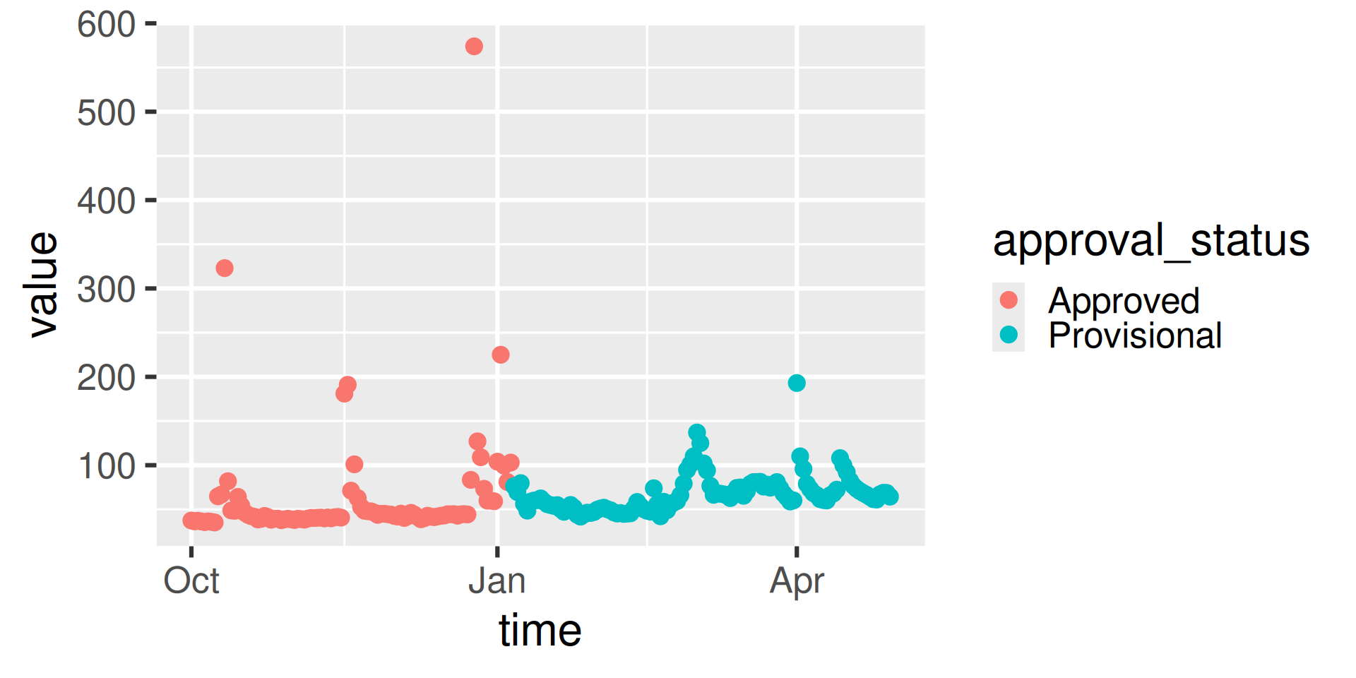
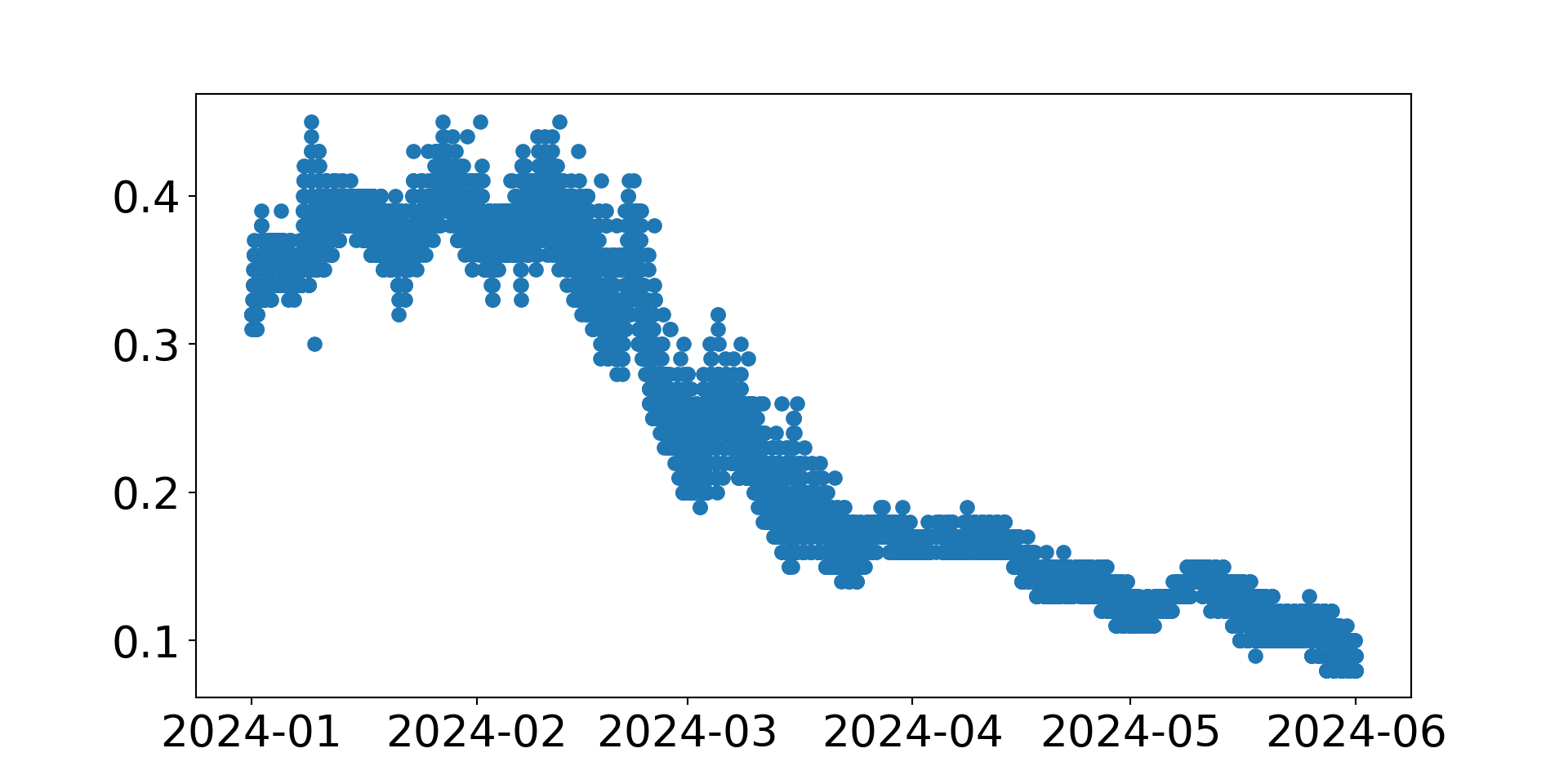
Let’s use matplotlib to visualize the data.
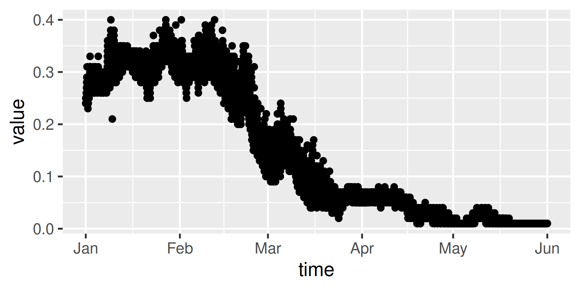
Water Data API Notes: Argument input
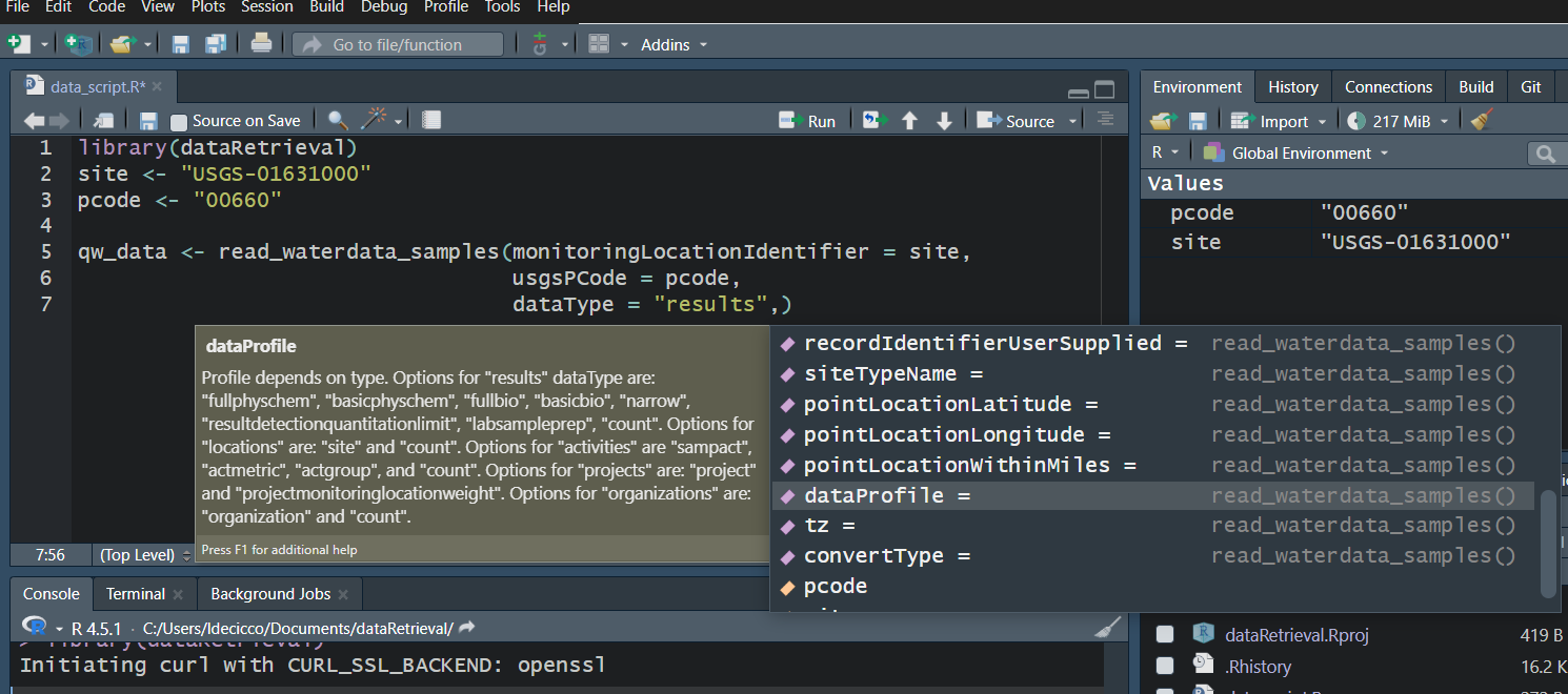
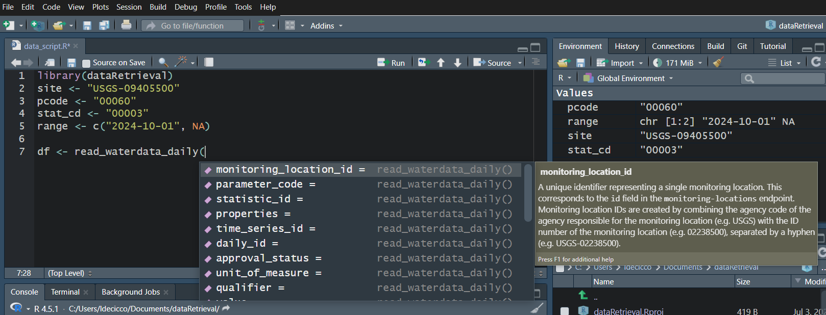
Use your “tab” key!
Workflow 2: Discrete data for known site
Use your “tab” key!