Using the waterdata module to pull data from the USGS Water Data APIs

The waterdata module replaces the nwis module for accessing USGS water data. It leverages the Water Data APIs to download metadata, daily values, and instantaneous values.

While the specifics of this transition timeline are opaque, it is advised to switch to the new functions as soon as possible to reduce unexpected interruptions in your workflow.

As always, please report any issues you encounter on our Issues page. If you have questions or need help, please reach out to us at comptools@usgs.gov.

Prerequisite: Get your Water Data API key

We highly suggest signing up for your own API key here to afford yourself higher rate limits and more reliable access to the data. If you opt not to register for an API key, then the number of requests you can make to the Water Data APIs is considerably lower, and if you share an IP address across users or workflows, you may hit those limits even faster. Luckily, registering for an API key is free and easy.

Once you’ve copied your API key and saved it in a safe place, you can set it as an environment variable in your python script for the current session:

import os
os.environ['API_USGS_PAT'] = 'your_api_key_here'

Note that the environment variable name is API_USGS_PAT, which stands for “API USGS Personal Access Token”.

If you’d like a more permanent, repository-specific solution, you can use the python-dotenv package to read your API key from a .env file in your repository root directory, like this:

!pip install python-dotenv # only run this line once to install the package in your environment
from dotenv import load_dotenv
load_dotenv()  # this will load the environment variables from the .env file

Make sure your .env file contains the following line:

API_USGS_PAT=your_api_key_here

Also, do not commit your .env file to version control, as it contains sensitive information. You can add it to your .gitignore file to prevent accidental commits.

Lay of the Land

Now that your API key is configured, it’s time to take a 10,000-ft view of the functions in the waterdata module.

Metadata endpoints

These functions retrieve metadata tables that can be used to refine your data requests.

• get_reference_table() - Not sure which parameter code you’re looking for, or which hydrologic unit your study area is in? This function will help you find the right input values for the data endpoints to retrieve the information you want.

• get_codes() - Similar to get_reference_table(), this function retrieves dataframes containing available input values that correspond to the Samples water quality database.

Data endpoints

• get_daily() - Daily values for monitoring locations, parameters, stat codes, and more.

• get_continuous() - Instantaneous values for monitoring locations, parameters, statistical codes, and more.

• get_monitoring_locations()- Monitoring location information such as name, monitoring location ID, latitude, longitude, huc code, site types, and more.

• get_time_series_metadata() - Timeseries metadata across monitoring locations, parameter codes, statistical codes, and more. Can be used to answer the question: what types of data are collected at my site(s) of interest and over what time period are/were they collected?

• get_latest_continuous() - Latest instantaneous values for requested monitoring locations, parameter codes, statistical codes, and more.

• get_latest_daily() - Latest daily values for requested monitoring locations, parameter codes, statistical codes, and more.

• get_field_measurements() - Physically measured values (a.k.a discrete) of gage height, discharge, groundwater levels, and more for requested monitoring locations.

• get_samples() - Discrete water quality sample results for monitoring locations, observed properties, and more.

A few key tips

• You’ll notice that each of the data functions have many unique inputs you can specify. DO NOT specify too many! Specify just enough inputs to return what you need. But do not provide redundant geographical or parameter information as this may slow down your query and lead to errors.

• Each function returns a Tuple, containing a dataframe and a Metadata class. If you have geopandas installed in your environment, the dataframe will be a GeoDataFrame with a geometry included. If you do not have geopandas, the dataframe will be a pandas dataframe with the geometry contained in a coordinates column. The Metadata object contains information about your query, like the query url.

• If you do not want to return the geometry column, use the input skip_geometry=True.

• All of these functions (except get_samples()) have a limit argument, which signifies the number of rows returned with each “page” of data. The Water Data APIs use paging to chunk up large responses and send data most efficiently to the requester. The waterdata functions collect the rows of data from each page and combine them into one final dataframe at the end. The default and maximum limit per page is 50,000 rows. In other words, if you request 100,000 rows of data from the database, it will return all the data in 2 pages, and each page counts as a “request” using your API key. If you were to change the argument to limit=10000, then each page returned would contain 10,000 rows, and it would take 10 requests/pages to return the total 100,000 rows. In general, there is no need to adjust the limit argument. However, if you are working with slow internet speeds, adjusting the limit argument may reduce chances of failures due to bandwidth.

• You can find some other helpful tips in the Water Data API documentation.

Examples

Let’s get into some examples using the functions listed above. First, we need to load the waterdata module and a few other packages and functions to go through the examples. To run the entirety of this notebook, you will need to install dataretrieval, matplotlib, and geopandas packages (plus dependencies). matplotlib is needed to create the plots, and geopandas is needed to create the interactive maps.

Note that if you use conda rather than pip, you do not need to install folium and mapclassify separately, as they are included in the conda-forge geopandas install.

!pip install dataretrieval
!pip install matplotlib
!pip install geopandas
!pip install folium
!pip install mapclassify

import pandas as pd
import matplotlib.pyplot as plt
import matplotlib.dates as mdates
import matplotlib.ticker as mtick
from IPython.display import display
from datetime import datetime, timedelta
from datetime import date
from dateutil.relativedelta import relativedelta
from dataretrieval import waterdata

pcodes,metadata = waterdata.get_reference_table("parameter-codes")
display(pcodes.head())

	parameter_code	parameter_name	unit_of_measure	parameter_group_code	parameter_description	medium	statistical_basis	time_basis	weight_basis	particle_size_basis	sample_fraction	temperature_basis	epa_equivalence
0	00001	Xsec loc, US from rb	ft	INF	Location in cross section, distance from right...	None	None	None	None	None	None	None	Agree
1	00002	Xsec loc, US from rb	%	INF	Location in cross section, distance from right...	None	None	None	None	None	None	None	Agree
2	00003	Sampling depth	ft	INF	Sampling depth, feet	None	None	None	None	None	None	None	Agree
3	00004	Stream width	ft	PHY	Stream width, feet	None	None	None	None	None	None	None	Agree
4	00005	Loctn in X-sec,depth	%	INF	Location in cross section, fraction of total d...	None	None	None	None	None	Total	None	Agree

Let’s say we want to find all parameter codes relating to streamflow discharge. We can use some string matching to find applicable codes.

streamflow_pcodes = pcodes[pcodes['parameter_name'].str.contains('streamflow|discharge', case=False, na=False)]
display(streamflow_pcodes[['parameter_code', 'parameter_name']])

	parameter_code	parameter_name
42	00060	Discharge
43	00061	Discharge, instant.
479	01351	Streamflow, severity
769	04122	Bedload discharge, daily mean
1701	30208	Discharge
1702	30209	Instantaneous Discharge
3704	50042	Discharge
8838	62856	Discharge, storm event peak
13745	70227	Direction,StreamFlow
13952	72122	Discharge, storm event median
13953	72123	Discharge, storm event mean
13967	72137	Discharge,tide fltrd
13968	72138	Discharge,tide fltrd
13969	72139	Discharge,tide fltrd
14006	72177	Discharge, GW
14070	72243	Discharge
14085	72258	Discharge factor
14099	72272	Discharge, cumul
14260	72433	Discharge, cumulative
14261	72434	Discharge, cumulative
14296	74082	Streamflow, daily
14643	81380	Discharge velocity
14644	81381	Discharge duration
14686	81799	Discharge, sample mean
18706	99060	Discharge
18707	99061	Discharge, instantaneous

Interesting that there are so many different streamflow-related parameter codes! Going on experience, let’s use the most common one, 00060, which is “Discharge, cubic feet per second”.

Timeseries metadata

Now that we know which parameter code we want to use, let’s find all the stream monitoring locations that have recent discharge data and at least 10 years of daily values in the state of Nebraska. We will use the waterdata.get_time_series_metadata() function to suss out which sites fit the bill. This function will return a row for each timeseries that matches our inputs. It doesn’t contain the daily discharge values themselves, just information about that timeseries.

First, let’s get our expected date range in order. Note that the waterdata functions are capable of taking in bounded and unbounded date and datetime ranges. In this case, we want the start date of the discharge timeseries to be no more recent than 10 years ago, and we want the end date of the timeseries to be from at most a week ago. We can use the notation {date}/.. to mean that we want all timeseries that end a week ago or more recently. Similarly, we can use the notation ../{date} to mean we want all timeseries that started at least 10 years ago (and thus likely have at least 10 years of data).

ten_years_ago =(date.today() - relativedelta(years=10)).strftime("%Y-%m-%d")
one_week_ago = (datetime.now() - timedelta(days=7)).date().strftime("%Y-%m-%d")

We will also use the skip_geometry argument in our timeseries metadata call. By default, most waterdata functions return a geometry column containing the monitoring location’s coordinates. This is a really cool feature that we will use later, but for this particular data pull, we don’t need it. Setting skip_geometry=True makes the returned dataframe smaller and more efficient.

NE_discharge,_ = waterdata.get_time_series_metadata(
    state_name="Nebraska",
    parameter_code='00060',
    begin=f"../{ten_years_ago}",
    end=f"{one_week_ago}/..",
    skip_geometry=True
)

display(NE_discharge.sort_values("monitoring_location_id").head())
print(f"There are {len(NE_discharge['monitoring_location_id'].unique())} sites with recent discharge data available in the state of Nebraska")

	time_series_id	unit_of_measure	parameter_name	parameter_code	statistic_id	hydrologic_unit_code	state_name	last_modified	begin	end	...	end_utc	computation_period_identifier	computation_identifier	thresholds	sublocation_identifier	primary	monitoring_location_id	web_description	parameter_description	parent_time_series_id
28	2daeaac402fb46e594ad265d1fed145c	ft^3/s	Discharge	00060	00003	101701040305	Nebraska	2026-01-22 06:30:18.666975	1957-10-01 00:00:00.000001	2026-01-20 00:00:00.000001	...	2026-01-20 06:00:00+00:00	Daily	Mean	[]	None	Primary	USGS-06453600	None	Discharge, cubic feet per second	c8f66a81be244941a4c8975ac4393f57
160	c8f66a81be244941a4c8975ac4393f57	ft^3/s	Discharge	00060	00011	101701040305	Nebraska	2026-01-22 05:30:10.892931	1990-10-01 05:30:00.000001	2026-01-22 05:15:00.000001	...	2026-01-22 11:15:00+00:00	Points	Instantaneous	[{'Name': 'Peak of record discharge on March 2...	None	Primary	USGS-06453600	Discharge from Primary Sensor	Discharge, cubic feet per second	None
131	a661caa558244bf8a054018ccae0553a	ft^3/s	Discharge	00060	00003	101500040905	Nebraska	2026-01-22 06:59:23.720590	1945-10-01 00:00:00.000001	2026-01-21 00:00:00.000001	...	2026-01-21 06:00:00+00:00	Daily	Mean	[]	None	Primary	USGS-06461500	None	Discharge, cubic feet per second	9d41bfe5d9374b998cb9c93310bbbdd8
125	9d41bfe5d9374b998cb9c93310bbbdd8	ft^3/s	Discharge	00060	00011	101500040905	Nebraska	2026-01-22 09:59:12.152814	1991-05-17 05:00:00.000001	2026-01-22 09:45:00.000001	...	2026-01-22 15:45:00+00:00	Points	Instantaneous	[{'Name': 'VERY HIGH', 'Type': 'ThresholdAbove...	None	Primary	USGS-06461500	None	Discharge, cubic feet per second	None
65	58fcf157597f4f8f9b351312a1993e05	ft^3/s	Discharge	00060	00003	101500041309	Nebraska	2026-01-22 06:50:25.193316	1948-05-01 00:00:00.000001	2026-01-21 00:00:00.000001	...	2026-01-21 06:00:00+00:00	Daily	Mean	[]	None	Primary	USGS-06463500	None	Discharge, cubic feet per second	f5f7a38d1ad548dbb6f4cb876f9833a5

5 rows × 21 columns

There are 101 sites with recent discharge data available in the state of Nebraska

In the dataframe above, we are looking at 5 timeseries returned, ordered by monitoring location. You can also see that the first two rows show two different kinds of discharge for the same monitoring location: a mean daily discharge timeseries (with statistic id 00003, which represents “mean”) and an instantaneous discharge timeseries (with statistic id 00011, which represents “points” or “instantaneous” values). Look closely and you may also notice that the parent_timeseries_id column for daily mean discharge matches the time_series_id for the instantaneous discharge. This is because once instantaneous measurements began at the site, they were used to calculate the daily mean.

Monitoring locations

Now that we know which sites have recent discharge data, let’s find stream sites and plot them on a map. We will use the waterdata.get_monitoring_locations() function to grab more metadata about these sites.

We can feed the unique monitoring location IDs from NE_discharge into the get_monitoring_locations() function to get the metadata for just those sites. However, there is a limit to the number of IDs that can be passed in one call to the API. Further down in this notebook, you’ll see an example where we successfully feed all ~100 IDs in one call to the API. However, for demonstration purposes, we will split the list of monitoring location IDs into a few chunks of 50 sent to the API and stitch the resulting dataframes together. A loose rule of thumb is to keep the number of IDs below 200, but this exact number will depend on the typical length of each monitoring location ID (i.e. if your monitoring location IDs are > 13 characters long: “USGS-XXXXXXXX”+, you will need to feed in less than 200 at a time).

chunk_size=50
site_list = NE_discharge['monitoring_location_id'].unique().tolist()
chunks = [site_list[i:i + chunk_size] for i in range(0, len(site_list), chunk_size)]
NE_locations = pd.DataFrame()
for site_group in chunks:
        try:
            chunk_data,_ = waterdata.get_monitoring_locations(
                monitoring_location_id=site_group,
                site_type_code="ST"
            )
            if not chunk_data.empty:
                NE_locations = pd.concat([NE_locations, chunk_data])
        except Exception as e:
            print(f"Chunk failed: {e}")

display(NE_locations[["monitoring_location_id", "monitoring_location_name", "hydrologic_unit_code"]].head())

	monitoring_location_id	monitoring_location_name	hydrologic_unit_code
0	USGS-06453600	Ponca Creek at Verdel, Nebr.	101701040305
1	USGS-06463720	Niobrara River at Mariaville, Nebr.	101500041506
2	USGS-06600900	South Omaha Creek at Walthill, Nebr.	102300010103
3	USGS-06610770	Big Papillion Creek at Q Street at Omaha, Nebr.	102300060205
4	USGS-06610795	Papillion Creek at Fort Crook, Nebr.	102300060206

That took a little bit of work to loop through the site chunks and bind the data back together. Admittedly, there may be times where chunking and iterating might be the most efficient workflow. But in this particular case, we have a less onerous option available: get_monitoring_locations() has a state_name argument. It will likely be faster to pull all stream sites for Nebraska and then filter down to the sites present in the timeseries dataframe: no iteration needed. Let’s try this too.

NE_locations,_ = waterdata.get_monitoring_locations(
    state_name="Nebraska",
    site_type_code="ST"
    )

NE_locations_discharge = NE_locations.loc[NE_locations['monitoring_location_id'].isin(NE_discharge['monitoring_location_id'].unique().tolist())]
display(NE_locations_discharge[["monitoring_location_id", "monitoring_location_name", "hydrologic_unit_code"]].head())

	monitoring_location_id	monitoring_location_name	hydrologic_unit_code
14	USGS-06453600	Ponca Creek at Verdel, Nebr.	101701040305
44	USGS-06461500	Niobrara River near Sparks, Nebr.	101500040905
61	USGS-06463500	Long Pine Creek near Riverview, Nebr.	101500041309
63	USGS-06463720	Niobrara River at Mariaville, Nebr.	101500041506
79	USGS-06465500	Niobrara River near Verdel, Nebr.	101500071004

If you have geopandas installed, the function will return a GeoDataFrame with a geometry column containing the monitoring locations’ coordinates. You can use gpd.explore() to view your geometry coordinates on an interactive map. We will demo this functionality below (Hover over the site points to see all the columns returned from waterdata.get_monitoring_locations()). If you don’t have geopandas installed, dataretrieval will return a regular pandas DataFrame with coordinate columns instead.

NE_locations_discharge.set_crs(crs="WGS84").explore()

Make this Notebook Trusted to load map: File -> Trust Notebook

Latest daily and instantaneous values

Now that we know which sites in Nebraska have recent discharge data, and we know where they are located, we can start downloading some actual flow values. Let’s start with some of the most “lightweight” functions, waterdata.get_latest_daily() and waterdata.get_latest_continuous(), which will return only the latest value for each monitoring location requested.

Recall from above, we are working with ~100 sites with discharge data. Conveniently, the waterdata functions are usually pretty good at handling requests of up to ~200 monitoring locations. However, if you have more than 200, you may be better off chopping up your list of sites into a few lists that you loop over.

latest_dv,_ = waterdata.get_latest_daily(
    monitoring_location_id=NE_locations_discharge['monitoring_location_id'].tolist(),
    parameter_code="00060",
    statistic_id="00003"
)
display(latest_dv.head())

	geometry	time_series_id	monitoring_location_id	parameter_code	statistic_id	time	value	unit_of_measure	approval_status	qualifier	last_modified	latest_daily_id
0	POINT (-97.42603 42.00378)	8925986a50c64185a9ffc2a4a57f6938	USGS-06799000	00060	00003	2026-01-18	NaN	ft^3/s	Provisional	[ICE]	2026-01-22 14:15:37.133128+00:00	243651b2-f705-4679-bb0d-f5fe24dbfe90
1	POINT (-100.10087 41.8311)	bdcca64f4fe24be08056ab5d75cc12cc	USGS-06775500	00060	00003	2026-01-20	NaN	ft^3/s	Provisional	[ICE]	2026-01-21 16:29:19.413284+00:00	723bc7f7-f099-4de5-8813-714a12e989a0
2	POINT (-98.44636 41.20394)	ee305abb2cd54649987f8a03b895827e	USGS-06785000	00060	00003	2026-01-20	NaN	ft^3/s	Provisional	[ICE]	2026-01-21 19:44:24.191900+00:00	1f9b312c-c086-414b-92d6-380cd11c69bc
3	POINT (-99.8601 41.94174)	fa70c721512148b69cee7f253431ad4f	USGS-06785500	00060	00003	2026-01-20	NaN	ft^3/s	Provisional	[ICE]	2026-01-21 08:22:37.974618+00:00	92e08d3d-2096-430e-b769-40ed3604bbf4
4	POINT (-99.3797 41.77693)	f2077ca2dde64732bfb9cfc185837885	USGS-06786000	00060	00003	2026-01-20	NaN	ft^3/s	Provisional	[ICE]	2026-01-21 08:21:58.427337+00:00	4e965e06-2d0e-4d53-81aa-28828b13ccf1

Note that because these measurements are less than a week old, most of them are still tagged as “Provisional” in the approval_status column. Some may also be missing values in the value column. You can often check the qualifier column for clues as to why a value is missing, or additional information specific to that measurement. Let’s map out the monitoring locations again and color the points based on the latest daily value.

latest_dv['date'] = latest_dv['time'].astype(str)
latest_dv[['geometry', 'monitoring_location_id', 'date', 'value', 'unit_of_measure']].set_crs(crs="WGS84").explore(column='value', tiles='CartoDB dark matter', cmap='YlOrRd', scheme=None, legend=True)

Make this Notebook Trusted to load map: File -> Trust Notebook

Let’s do the same routine with waterdata.get_latest_continuous(), but note that we do not need to specify the statistic_id: all instantaneous values have the statistical code “00011”.

latest_instantaneous,_ = waterdata.get_latest_continuous(
    monitoring_location_id=NE_locations_discharge['monitoring_location_id'].tolist(),
    parameter_code="00060"
)

latest_instantaneous['datetime'] = latest_instantaneous['time'].astype(str)
latest_instantaneous[['geometry', 'monitoring_location_id', 'datetime', 'value', 'unit_of_measure']].set_crs(crs="WGS84").explore(column='value', cmap='YlOrRd', scheme=None, legend=True)

Make this Notebook Trusted to load map: File -> Trust Notebook

Daily and continuous values datasets

While the “latest” functions might be helpful for “realtime” or “current” dashboards or reports, many users desire to work with a complete timeseries of daily summary (min, max, mean) or instantaneous values for their analyses. For these workflows, waterdata.get_daily() and waterdata.get_continuous() are helpful.

Using our current example, let’s say that you want to compare daily and instantaneous discharge values for monitoring locations along the Missouri River in Nebraska.

missouri_river_sites = NE_locations_discharge.loc[NE_locations_discharge['monitoring_location_name'].str.contains("Missouri")]
display(missouri_river_sites[[
    'county_name',
    'site_type',
    'monitoring_location_id',
    'monitoring_location_name',
    'drainage_area',
    'altitude'
    ]])

	county_name	site_type	monitoring_location_id	monitoring_location_name	drainage_area	altitude
111	Dakota County	Stream	USGS-06486000	Missouri River at Sioux City, IA	314600.0	1057.42
136	Douglas County	Stream	USGS-06610000	Missouri River at Omaha, NE	322800.0	948.97
675	Otoe County	Stream	USGS-06807000	Missouri River at Nebraska City, NE	410000.0	905.61
687	Richardson County	Stream	USGS-06813500	Missouri River at Rulo, NE	414900.0	838.16

Currently, users may only request 3 years or less of continuous data in one pull. For this example, let’s pull the last 1 year of daily mean values and instantaneous values for these Missouri River sites. We’ll skip pulling geometry in the waterdata.get_daily() function; the waterdata.get_continuous() function does not return geometry at all to economize the size of the dataset returned.

one_year_ago = (date.today() - relativedelta(years=1)).strftime("%Y-%m-%d")
missouri_site_ids = missouri_river_sites['monitoring_location_id'].tolist()
missouri_site_names = missouri_river_sites['monitoring_location_name'].tolist()

daily_values,_ = waterdata.get_daily(
    monitoring_location_id=missouri_site_ids,
    parameter_code="00060",
    statistic_id="00003", # mean daily value
    time=f"{one_year_ago}/..",
    skip_geometry=True
)

instantaneous_values,_ = waterdata.get_continuous(
    monitoring_location_id=missouri_site_ids,
    parameter_code="00060",
    time=f"{one_year_ago}T00:00:00Z/.."
)

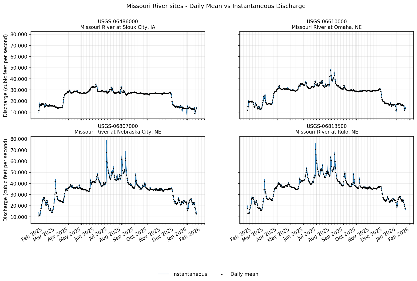
With these two datasets, let’s plot daily and instantaneous discharge values for the four Missouri River sites using matplotlib. We will plot each site on a different subplot, with instantaneous values represented by a blue line and daily mean values represented by black points.

fig, axes = plt.subplots(2, 2, figsize=(14, 8), dpi=150, sharex=False, sharey=True)
axes = axes.ravel()

# Y-axis formatter (with thousands separators)
tick_fmt = mtick.StrMethodFormatter('{x:,.0f}')

for ax, site, site_name in zip(axes, missouri_site_ids, missouri_site_names):
    # Filter per site & sort by time
    inst = instantaneous_values.loc[instantaneous_values['monitoring_location_id'] == site, ["time", "value"]].sort_values("time")
    daily = daily_values.loc[daily_values['monitoring_location_id'] == site, ["time", "value"]].sort_values("time")

    # Instantaneous (line)
    ax.plot(
        inst["time"], inst["value"],
        color="#1f77b4", lw=1.0, label="Instantaneous", zorder=1
    )

    # Daily mean (black dots)
    ax.scatter(
        daily["time"], daily["value"],
        c="black", s=2, label="Daily mean", zorder=2
    )

    # Axes styling
    ax.set_title(f"{site}\n{site_name}", fontsize=10)
    ax.grid(True, which="both", alpha=0.25)
    ax.yaxis.set_major_formatter(tick_fmt)

    # Time ticks
    ax.xaxis.set_major_locator(mdates.MonthLocator())
    ax.xaxis.set_major_formatter(mdates.DateFormatter("%b %Y"))
    ax.xaxis.set_minor_locator(mdates.WeekdayLocator(byweekday=mdates.MO))

# Common axis labels (left y on both left subplots; x labels on bottom row)
axes[0].set_ylabel("Discharge (cubic feet per second)")
axes[2].set_ylabel("Discharge (cubic feet per second)")
axes[2].set_xlabel("")
axes[3].set_xlabel("")

handles, labels = axes[-1].get_legend_handles_labels()
fig.legend(handles, labels, loc="lower center", ncol=2, frameon=False)
fig.suptitle(f"Missouri River sites - Daily Mean vs Instantaneous Discharge")
fig.autofmt_xdate()

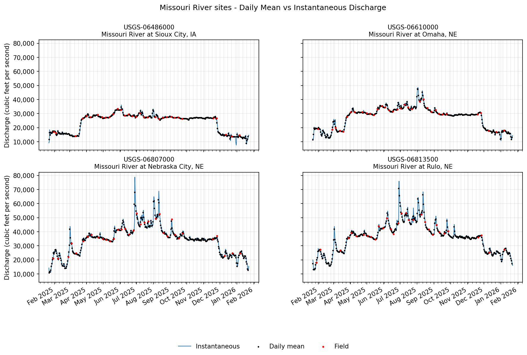
Field values

Finally, let’s see if there are any discharge field measurements for these sites. These are manually recorded measurements (by a human), often used during calibration checks. We will use waterdata.get_field_measurements() to check. More commonly, a user would head to this function to gather groundwater level data, which are categorized as field measurements.

field_measurements,_ = waterdata.get_field_measurements(
    monitoring_location_id=missouri_site_ids,
    parameter_code="00060",
    time=f"{one_year_ago}T00:00:00Z/.."
)
display(field_measurements.head())

	geometry	field_visit_id	parameter_code	monitoring_location_id	observing_procedure_code	observing_procedure	value	unit_of_measure	time	qualifier	vertical_datum	approval_status	measuring_agency	last_modified	field_measurement_id
0	POINT (-95.42175 40.05206)	0c25bcf0-f8f9-4044-b051-bb73bd19498c	00060	USGS-06813500	Z	Acoustic Doppler Current Profiler	18000	ft^3/s	2025-01-28 19:19:42+00:00	None	None	Approved	USGS	2025-06-13 18:55:43.542508+00:00	844b8fa8-de6e-4d42-aed2-be587511305b
1	POINT (-95.84708 40.68181)	8d9e937b-7e60-4106-9b3d-dcc32c7323b1	00060	USGS-06807000	Z	Acoustic Doppler Current Profiler	21100	ft^3/s	2025-01-29 16:37:11+00:00	None	None	Approved	USGS	2025-06-17 19:41:06.711794+00:00	8d21a28b-e818-4cff-a6cc-9448f298eb7a
2	POINT (-96.41308 42.48619)	9c2d9eb3-de9d-44d8-aca7-aa46de633040	00060	USGS-06486000	Z	Acoustic Doppler Current Profiler	16900	ft^3/s	2025-01-30 17:17:12+00:00	None	None	Approved	USGS	2025-06-16 20:30:51.750716+00:00	4f8ffeda-3d65-4219-9f65-6759beb27f82
3	POINT (-95.92325 41.25906)	df9e30ec-5f70-431c-97f3-fc0ebd31044f	00060	USGS-06610000	Z	Acoustic Doppler Current Profiler	19100	ft^3/s	2025-01-31 16:48:25+00:00	None	None	Approved	USGS	2025-06-17 19:35:53.102935+00:00	dc9a2b8b-932c-4053-b858-c1f22d4ccaa7
4	POINT (-96.41308 42.48619)	e9a04cf4-54fd-45f2-b742-d526250cae66	00060	USGS-06486000	Z	Acoustic Doppler Current Profiler	16300	ft^3/s	2025-02-03 17:10:55+00:00	None	None	Approved	USGS	2025-06-16 20:30:51.750716+00:00	06d4b3c4-ca1e-4c1b-bf73-a80c91a420f1

Hey! We have some! Let’s add these to our plots from above. We’ll loop through each monitoring location plot and add in field measurements as red points.

for ax, site in zip(axes, missouri_site_ids):
    field = field_measurements.loc[
        field_measurements['monitoring_location_id'] == site, ["time", "value"]
    ].sort_values("time")

    ax.scatter(
        field["time"], field["value"],
        c="red", s=4, label="Field", zorder=3
    )

# Remove any existing figure-level legends
for leg in fig.legends:
    leg.remove()
handles, labels = axes[-1].get_legend_handles_labels()
fig.legend(handles, labels, loc="lower center", ncol=3, frameon=False)

# Redraw the figure
fig.canvas.draw_idle()
fig

Additional Resources

The USGS Water Data APIs belong to the Water Data for the Nation (WDFN) group of applications and tools. These products exist under the broader National Water Information System (NWIS) program. Check out the links below for more information on the USGS Water Data APIs and other ways to download or view USGS water data:

• Water Data APIs Home

• Get an API Key

• Water Data API OGC Endpoint Catalog

• Water Data Download Form

• Water Data for the Nation Home

• Water Data for the Nation Feedback Form

• R dataRetrieval package

• WDFN Blog Post on NWISWeb Decommissioning Timeline