National trends in peak annual streamflow

Introduction

This notebook demonstrates a slightly more advanced application of the dataretrieval.waterdata module: assembling a dataset of historical annual peak streamflow and regressing peak discharge against time to look for trends — not at a single station, but across many.

Setup

Before we begin any analysis, we’ll need to set up our environment by importing a few modules.

import numpy as np
import pandas as pd
from scipy import stats

from dataretrieval import waterdata

Basic usage

The waterdata module is the recommended interface to USGS water data and replaces the deprecated nwis module. Annual peak streamflow is retrieved with waterdata.get_peaks(), which returns a pandas data frame and a metadata object. To get started we need a monitoring location ID, a parameter code, and (optionally) a time window.

# download annual peaks (discharge, parameter 00060) from a single site
df, md = waterdata.get_peaks(
    monitoring_location_id="USGS-03339000",
    parameter_code="00060",
    time="1970-01-01/..",
)
df.head()

Retrieving: peaks · 1 page · 56 rows
No API key detected — register for higher rate limits at https://api.waterdata.usgs.gov/signup/

	geometry	time_series_id	monitoring_location_id	parameter_code	unit_of_measure	value	last_modified	time	water_year	year	month	day	time_of_day	peak_since	qualifier	peak_id
0	POINT (-87.59761 40.10108)	1587ac4ee41d4f6b9debe9724e8ddb79	USGS-03339000	00060	ft^3/s	16300	2026-04-28 09:40:12.927288+00:00	1970-04-20	1970	1970	4	20	NaN	None	[UNKNOWNREGULATION]	5282b66f-ee19-43d9-b772-936da66a968d
1	POINT (-87.59761 40.10108)	1587ac4ee41d4f6b9debe9724e8ddb79	USGS-03339000	00060	ft^3/s	8910	2026-04-28 09:40:12.927288+00:00	1971-02-05	1971	1971	2	5	NaN	None	[UNKNOWNREGULATION]	935a7d88-6e6c-4b80-b6a2-20b909d6e67f
2	POINT (-87.59761 40.10108)	1587ac4ee41d4f6b9debe9724e8ddb79	USGS-03339000	00060	ft^3/s	9240	2026-04-28 09:40:12.927288+00:00	1972-04-22	1972	1972	4	22	NaN	None	[UNKNOWNREGULATION]	69975ecd-959a-46bc-a221-815c947a76b6
3	POINT (-87.59761 40.10108)	1587ac4ee41d4f6b9debe9724e8ddb79	USGS-03339000	00060	ft^3/s	16600	2026-04-28 09:40:12.927288+00:00	1973-04-23	1973	1973	4	23	NaN	None	[UNKNOWNREGULATION]	55fc2bdd-fc45-44d5-b291-6767e5e44ff6
4	POINT (-87.59761 40.10108)	1587ac4ee41d4f6b9debe9724e8ddb79	USGS-03339000	00060	ft^3/s	19500	2026-04-28 09:40:12.927288+00:00	1974-06-23	1974	1974	6	23	NaN	None	[UNKNOWNREGULATION]	c202f21a-a940-418f-92d6-253598a16dd0

All we require for the trend analysis are the peak date (time), the monitoring location ID (monitoring_location_id), and the peak streamflow (value). The Water Data API returns a flat (single-index) data frame with one row per annual peak.

Preparing the regression

Next we’ll define a function that applies ordinary least squares to peak discharge versus time. After grouping the dataset by monitoring_location_id, we apply the regression per monitoring location. Each location’s result is returned as a row with the slope, y-intercept, p value, and standard error of the regression.

def peak_trend_regression(df):
    # convert peak dates to days since the first peak for the regression
    peak_date = pd.to_datetime(df["time"])
    peak_d = (peak_date - peak_date.min()) / np.timedelta64(1, "D")

    # normalize the peak discharge values
    value = (df["value"] - df["value"].mean()) / df["value"].std()

    slope, intercept, _r_value, p_value, std_error = stats.linregress(peak_d, value)

    return pd.Series(
        {
            "slope": slope,
            "intercept": intercept,
            "p_value": p_value,
            "std_error": std_error,
        }
    )

Preparing the analysis

def peak_trend_analysis(state_names, start_date):
    """
    state_names : list
        state names to include in the analysis, e.g. ["Illinois", "Indiana"].
    start_date : string
        the date to use as the beginning of the analysis (YYYY-MM-DD).
    """
    frames = []

    for state in state_names:
        # find stream gages in the state (keep the geometry for mapping)
        sites, _ = waterdata.get_monitoring_locations(
            state_name=state, site_type_code="ST"
        )
        # download annual peak discharge for those sites
        df, _ = waterdata.get_peaks(
            monitoring_location_id=sites["monitoring_location_id"].tolist(),
            parameter_code="00060",
            time=f"{start_date}/..",
        )
        # group the data by site and apply our regression
        temp = (
            df.groupby("monitoring_location_id")
            .apply(peak_trend_regression)
            .dropna()
        )
        # drop any insignificant results
        temp = temp[temp["p_value"] < 0.05]

        # join site geometry/metadata with the trend results; GeoDataFrame.merge
        # keeps the joined result spatial
        merged = sites.merge(
            temp, right_index=True, left_on="monitoring_location_id"
        )
        frames.append(merged)

    return pd.concat(frames, ignore_index=True)

Running the analysis for every state since 1970 would pull a large amount of data from the Water Data API and could burden the service. To keep this demo light, we run a single small state — Rhode Island — below.

# Download peak discharge for every stream gage in Rhode Island and run the
# trend regression on each. For larger states the async chunker (default
# concurrency 16) automatically fans the ``get_peaks`` call across many sites;
# Rhode Island is small enough to return in a single request.
start = "1970-01-01"
states = ["Rhode Island"]
final_df = peak_trend_analysis(state_names=states, start_date=start)
final_df.head()

Retrieving: monitoring-locations · 1 page · 351 rows
Retrieving: peaks · 1 page · 1,308 rows

	monitoring_location_id	geometry	agency_code	agency_name	monitoring_location_number	monitoring_location_name	district_code	country_code	country_name	state_code	...	well_constructed_depth	hole_constructed_depth	depth_source_code	revision_note	revision_created	revision_modified	slope	intercept	p_value	std_error
0	USGS-01114000	POINT (-71.41061 41.83399)	USGS	U.S. Geological Survey	01114000	MOSHASSUCK RIVER AT PROVIDENCE, RI	25	US	United States of America	44	...	NaN	NaN	None	WDR MA-RI, water years 1964-1973, annual peak ...	2017-11-13T06:00:00+00:00	2022-04-07T14:31:13.870000+00:00	0.000059	-0.588666	0.008529	0.000022
1	USGS-01115098	POINT (-71.60618 41.8526)	USGS	U.S. Geological Survey	01115098	PEEPTOAD BROOK AT ELMDALE RD NR NORTH SCITUATE...	25	US	United States of America	44	...	NaN	NaN	None	WDR MA-RI-03-01: Drainage area.	2017-11-13T06:00:00+00:00	NaN	0.000153	-0.846482	0.003592	0.000048
2	USGS-01115200	POINT (-71.75035 41.83121)	USGS	U.S. Geological Survey	01115200	SHIPPEE BROOK TRIBUTARY AT NORTH FOSTER, RI	25	US	United States of America	44	...	NaN	NaN	None	NaN	NaN	NaN	-0.001714	1.103788	0.000945	0.000130
3	USGS-01115800	POINT (-71.61284 41.64482)	USGS	U.S. Geological Survey	01115800	BIG RIVER NEAR NOOSENECK, RI	25	US	United States of America	44	...	NaN	NaN	None	NaN	NaN	NaN	-0.002928	0.707107	0.000000	0.000000
4	USGS-01117250	POINT (-71.53944 41.43222)	USGS	U.S. Geological Survey	01117250	BROWNS BROOK AT WAKEFIELD, RI	25	US	United States of America	44	...	NaN	NaN	None	NaN	NaN	NaN	-0.001486	1.175513	0.044431	0.000445

5 rows × 48 columns

The cell above ran the full analysis for a single small state (Rhode Island) and returned final_df — one row per gage whose peak-discharge trend is statistically significant (p_value < 0.05), carrying the regression slope, intercept, p-value, and standard error.

final_df pairs each station’s trend statistics with its monitoring-location metadata (monitoring_location_id, state_name, site_type_code, …) and, because we kept the locations’ geometry, a geometry column of point coordinates — so we can map the results directly.

Plotting the results

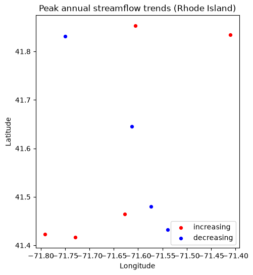
Because final_df is a GeoDataFrame, we can map the results directly with geopandas and matplotlib — no extra basemap stack required. Monitoring locations with increasing peak annual discharge are shown in red, and those with decreasing peaks in blue.

import matplotlib.pyplot as plt

# final_df is a GeoDataFrame, so its station points plot directly.
increasing = final_df[final_df["slope"] > 0]
decreasing = final_df[final_df["slope"] < 0]

fig, ax = plt.subplots(figsize=(8, 6))
if not increasing.empty:
    increasing.plot(ax=ax, color="red", markersize=18, label="increasing")
if not decreasing.empty:
    decreasing.plot(ax=ax, color="blue", markersize=18, label="decreasing")
ax.set_title(f"Peak annual streamflow trends ({', '.join(states)})")
ax.set_xlabel("Longitude")
ax.set_ylabel("Latitude")
ax.legend()
plt.show()