Compare discrete and sensor values
Robert M. Hirsch
Source:vignettes/Compare_QW_and_UV.Rmd
Compare_QW_and_UV.RmdComparing discrete sample values with their closest sensor value
One of the important steps in using high frequency sensor data is to check out how it compares to concentrations of the target analyte based on samples collected at the same location. The example case we will consider here is a site that has a large amount of discrete nitrate plus nitrite values (parameter code 00631) and a continuous nitrate sensor (parameter code 99133). In this discussion we will refer to the sample values as “qw” data and the sensor values as “uv” data. Throughout this discussion we will consider the qw values to be the “gold standard”, which is to say that they represent the measurements of concentration that we would like to have. USGS qw values are generally collected by devices that are iso-kinetic and the protocols used are designed to create a sample which is integrated horizontally and vertically over the full cross section, such that the average concentration in the sample collected, when multiplied by discharge, is an unbiased estimate of the flux of the analyte through the river.
Some of the things we might want to learn are these:
Are the uv data biased in relation to the qw data
What can we say about the distribution of errors (qw values minus uv values)
-
Determine if there may be a drift in the bias. The drift could be:
A changing bias over time
A changing bias as a function of river discharge
A bias that changes by season
A bias that is related to the uv value
Our goal here would be to create a statistical calibration model that allows the user to adjust the uv data so that it is approximately an unbiased estimate of the qw value at the time of the uv observation. This vignette covers some first steps in this process. More elaborate methods will certainly be needed, particularly those that might involve multiple uv variables measured at the same time, leading to a more complex calibration model. An example of that might be attempting to estimate total phosphorus concentration using a combination of sensor values (perhaps turbidity, pH, discharge,…). But we will leave that for another day.
The example problem we will work on here is for the Iowa River at Wappello, Iowa. The USGS site id is 05465500.
dataRetrieval
We want to work with the time period that starts with the first uv observations of nitrate and continues right up to the last uv observation in the record. When we retrieve the uv nitrate data we will also retrieve the associated discharge value. I already know (from looking at NWISweb) that the uv data started in 2009 and runs at least to the end of water year 2023.
First get the uv data
site_uv <- "05465500"
site_qw <-"USGS-05465500"
pcode_uv <- "99133"
pcode_qw <- "00631"
startDate <- "2009-01-01"
endDate <- "2023-09-30"
uv_data <- readNWISuv(site_uv, c(pcode_uv, "00060"), startDate = startDate, endDate = endDate)
# I don't want the row if it lacks the uv nitrate
uv_data <- uv_data[-which(is.na(uv_data$X_99133_00000)),]
# I also don't want the row if it lacks discharge
uv_data <- uv_data[-which(is.na(uv_data$X_00060_00000)),]
# now let's set the starting and ending on the actual period of record of the uv nitrate
start_sensor_date <- as.Date(min(uv_data$dateTime))
end_sensor_date <- as.Date(max(uv_data$dateTime))
# I also want to add a column for decimal year (handy for some graphing later)
uv_data$DecYear <- EGRET::decimalDate(uv_data$dateTime)
# before we look for the qw data let's take a quick look at the uv_data
numUv <- length(uv_data$agency_cd)
head(uv_data)
## agency_cd site_no dateTime X_00060_00000 X_00060_00000_cd
## 9502 USGS 05465500 2009-06-03 05:00:00 23300 A
## 9503 USGS 05465500 2009-06-03 05:15:00 23300 A
## 9504 USGS 05465500 2009-06-03 05:30:00 23300 A
## 9505 USGS 05465500 2009-06-03 05:45:00 23300 A
## 9506 USGS 05465500 2009-06-03 06:00:00 23300 A
## 9507 USGS 05465500 2009-06-03 06:15:00 23400 A
## X_99133_00000 X_99133_00000_cd tz_cd DecYear
## 9502 8.09 A UTC 2009.42
## 9503 8.13 A UTC 2009.42
## 9504 8.13 A UTC 2009.42
## 9505 8.13 A UTC 2009.42
## 9506 8.14 A UTC 2009.42
## 9507 8.13 A UTC 2009.42
cat("\n Number of values in the uv record is", numUv)##
## Number of values in the uv record is 335374
summary(uv_data)## agency_cd site_no dateTime
## Length :335374 Length :335374 Min. :2009-06-03 05:00:00
## N.unique : 1 N.unique : 1 1st Qu.:2014-05-25 18:33:45
## N.blank : 0 N.blank : 0 Median :2017-09-17 06:22:30
## Min.nchar: 4 Min.nchar: 8 Mean :2017-03-18 07:06:47
## Max.nchar: 4 Max.nchar: 8 3rd Qu.:2020-04-08 20:41:15
## Max. :2023-08-03 05:45:00
## X_00060_00000 X_00060_00000_cd X_99133_00000 X_99133_00000_cd
## Min. : 860 Length :335374 Min. : 0.000 Length :335374
## 1st Qu.: 4760 N.unique : 2 1st Qu.: 2.650 N.unique : 1
## Median : 9780 N.blank : 0 Median : 4.650 N.blank : 0
## Mean :12536 Min.nchar: 1 Mean : 4.677 Min.nchar: 1
## 3rd Qu.:17000 Max.nchar: 3 3rd Qu.: 6.430 Max.nchar: 1
## Max. :85100 Max. :30.700
## tz_cd DecYear
## Length :335374 Min. :2009
## N.unique : 1 1st Qu.:2014
## N.blank : 0 Median :2018
## Min.nchar: 3 Mean :2017
## Max.nchar: 3 3rd Qu.:2020
## Max. :2024Next we will get the qw data
qw_data <- readWQPqw(site_qw, pcode_qw, startDate = start_sensor_date,
                     endDate = end_sensor_date)
qw_data <- qw_data[-which(is.na(qw_data$ResultMeasureValue)),]
# and we will add a decimal year variable here too
qw_data$DecYear <- EGRET::decimalDate(qw_data$ActivityStartDateTime)
# and let's see what the qw_data data frame looks like
numQw <- length(qw_data$DecYear)
cat("\n Number of values in the qw record is", numQw)
##
## Number of values in the qw record is 238There are a large number of columns in qw_data, most are repetitive meta data. In the interest of brevity here we will just look at the first 10 values of the nitrate, the sampling date and time information, and DecYear. If one wanted to see more about the data frame one could do head(qw_data) and/or summary(qw_data).
The observations are not listed in chronological order. It would be a good idea to fix that problem here, because it could be problematic for later steps in the workflow.
qw_short <- data.frame(qw_data$ActivityStartDateTime, qw_data$DecYear, qw_data$ResultMeasureValue)
qw_short[1:10,]
## qw_data.ActivityStartDateTime qw_data.DecYear qw_data.ResultMeasureValue
## 1 2009-06-09 13:40:00 2009.437 8.11
## 2 2009-06-09 13:45:00 2009.437 8.04
## 3 2009-06-25 13:55:00 2009.481 6.99
## 4 2009-06-25 14:00:00 2009.481 6.94
## 5 2009-07-06 15:55:00 2009.511 6.51
## 6 2009-07-06 16:00:00 2009.511 6.49
## 7 2009-07-23 13:45:00 2009.558 6.10
## 8 2009-07-23 13:50:00 2009.558 6.12
## 9 2009-08-03 15:25:00 2009.588 3.62
## 10 2009-08-03 15:30:00 2009.588 3.68
summary(qw_short)## qw_data.ActivityStartDateTime qw_data.DecYear qw_data.ResultMeasureValue
## Min. :2009-06-09 13:40:00 Min. :2009 Min. : 0.070
## 1st Qu.:2011-05-07 21:00:00 1st Qu.:2011 1st Qu.: 3.518
## Median :2014-11-09 14:37:30 Median :2015 Median : 5.475
## Mean :2015-05-10 02:35:34 Mean :2015 Mean : 5.374
## 3rd Qu.:2018-11-25 23:45:00 3rd Qu.:2019 3rd Qu.: 6.980
## Max. :2023-06-22 15:45:00 Max. :2023 Max. :13.400
# put the qw_data data frame in chronological order
qw_data <- qw_data[order(qw_data$DecYear),]
# let's look at it again after sorting
qw_short <- data.frame(qw_data$ActivityStartDateTime, qw_data$DecYear, qw_data$ResultMeasureValue)
qw_short[1:10,]
## qw_data.ActivityStartDateTime qw_data.DecYear qw_data.ResultMeasureValue
## 1 2009-06-09 13:40:00 2009.437 8.11
## 2 2009-06-09 13:45:00 2009.437 8.04
## 3 2009-06-25 13:55:00 2009.481 6.99
## 4 2009-06-25 14:00:00 2009.481 6.94
## 5 2009-07-06 15:55:00 2009.511 6.51
## 6 2009-07-06 16:00:00 2009.511 6.49
## 7 2009-07-23 13:45:00 2009.558 6.10
## 8 2009-07-23 13:50:00 2009.558 6.12
## 9 2009-08-03 15:25:00 2009.588 3.62
## 10 2009-08-03 15:30:00 2009.588 3.68
rm(qw_short) # we aren't going to use it againThere is one additional issue with the qw_data. At the start there are pairs of samples that are taken a few minutes apart (replicates). A more advanced workflow would look for these and perhaps collapse them down to individual values. But for our puposes we have just left them in the data set.
The zero concentration values in the uv data set
The uv record does have some zero values and we need to be aware of that fact. Generally we don’t believe that concentrations ever go to zero, for a natural substance such as nitrate. We will want to try to find out how many zero values there are and we will want to learn a little more about them. Note that there are a total of 356,765 values and they span a total of a little more than 14 years. We might want to know how many zero values there are in the record. So we will create a subset of the data set that have values of zero and then take note of what fraction of the data are recorded as exactly zero. This vignette will not delve into problems of zeros or non-detects, but we need to recognize that new protocols are needed for dealing with this issue in the process of calibration of the sensors. This code will need to be improved to handle “less than” values and also handle zero values in the uv data. Note that we have not removed the zero values. If we decided in some later step to take logs of the concentration values we would have a problem and would have to deal with these zeros in an appropriate way.
# now let's make a subset of the data frame for only those with a value of 0.0
uv_data_zeros <- subset(uv_data, X_99133_00000 == 0.0)
numZeros <- length(uv_data_zeros$agency_cd)
cat("\n number of values that are exactly zero is", numZeros)
##
## number of values that are exactly zero is 225
fractZero <- format(100 * numZeros / numUv, digits = 2)
cat("percentage of unit values that are exactly zero is", fractZero, "%")
## percentage of unit values that are exactly zero is 0.067 %
rm(uv_data_zeros) # in future applications we might want to hold on to this subsetlooking at the uv concentration time series
par(tck = 0.03, las = 1, xaxs = "i", yaxs = "i", mar = c(5, 4, 5, 4))
staInfo <- attr(uv_data, "siteInfo")
title <- paste0(staInfo$station_nm, "   uv Parameter ", pcode_uv)
plot(uv_data$DecYear, uv_data$X_99133_00000, xlim = c(2009, 2024),
     ylim = c(0, 35), pch = "19", col = "red"
     , cex = 0.15, xlab = "", ylab = "Concentration, in mg/L",
     main = title, cex.lab = 1.1, cex.axis = 1.1,
     cex.main = 1.2)
axis(3, labels = FALSE)
axis(4, labels = FALSE)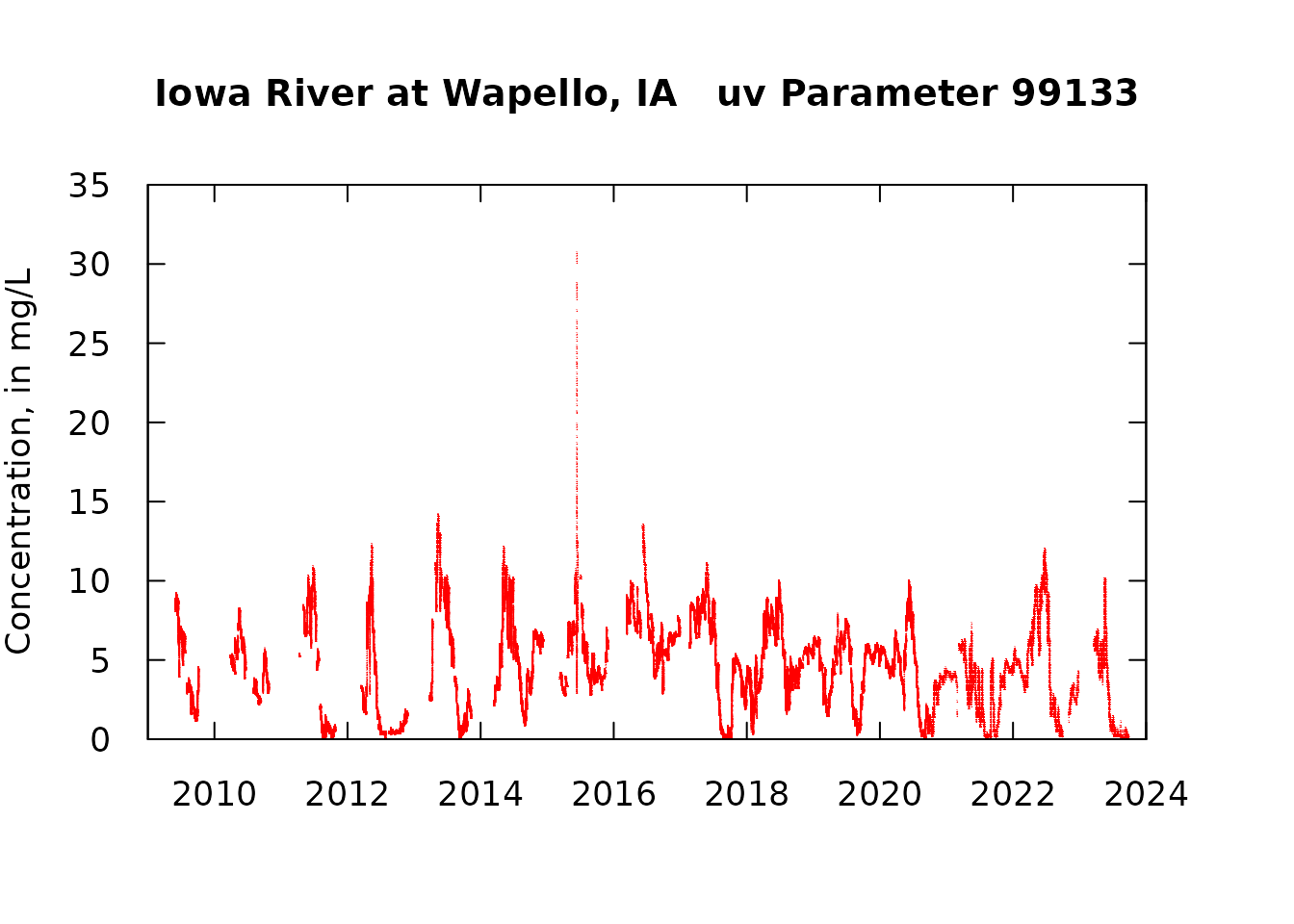
Now combined graphics of the two time series
par(tck = 0.03, las = 1, xaxs = "i", yaxs = "i", mar = c(5, 4, 5, 4))
staInfo <- attr(uv_data, "siteInfo")
title <- paste0(staInfo$station_nm, "   uv Parameter ", pcode_uv,"\nuv in red, sample values in green")
plot(uv_data$DecYear, uv_data$X_99133_00000, xlim = c(2009, 2024),
     ylim = c(0, 35), pch = "19", col = "red"
     , cex = 0.15, xlab = "", ylab = "Concentration, in mg/L",
     main = title, cex.lab = 1.1, cex.axis = 1.1,
     cex.main = 1.2)
points(qw_data$DecYear, qw_data$ResultMeasureValue, pch = 19, col = "green", cex = 0.5)
axis(3, labels = FALSE)
axis(4, labels = FALSE)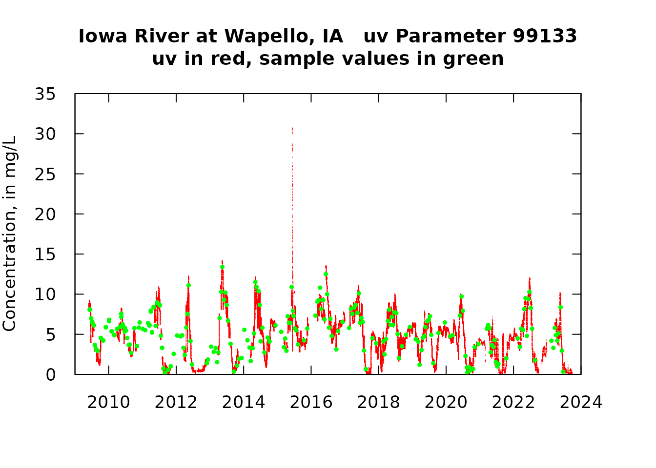
# Let's zero in on a smaller part of the record to get a better look
plot(uv_data$DecYear, uv_data$X_99133_00000, xlim = c(2018, 2019),
     ylim = c(0, 12), pch = "19", col = "red"
     , cex = 0.15, xlab = "", ylab = "Concentration, in mg/L",
     main = title, cex.lab = 1.1, cex.axis = 1.1,
     cex.main = 1.2)
points(qw_data$DecYear, qw_data$ResultMeasureValue, pch = 19, col = "green", cex = 0.8)
axis(3, labels = FALSE)
axis(4, labels = FALSE)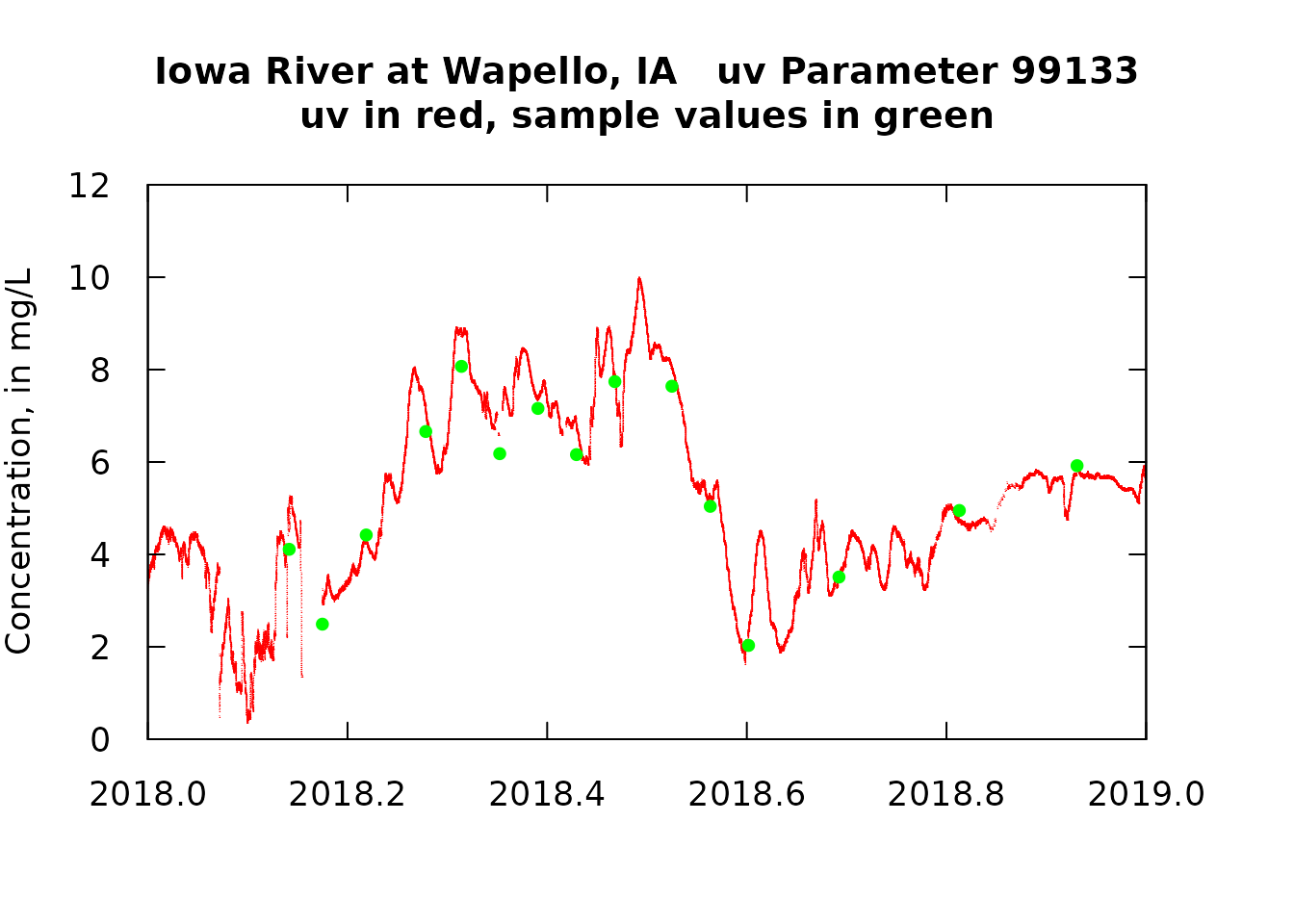
One of the things we see here is that there is a pretty good, but not perfect, match-up between the qw values and uv values. We also see that there are time gaps in the uv data set. What we want to do next is to focus on comparing the uv data with the qw data collected at about the same time. We will limit the matches of uv and qw data to only those that less than 12 hours apart. In most cases they will match up very closely in time (typically less than 15 minutes apart). What we would like to see is that these pairs of values are very similar and that on average the differences are very close to zero (i.e. the uv value is unbiased in relation to the qw value).
Doing the process of matching uv values with qw values
We would like to understand the differences between qw and uv values that are taken at about the same time. Here is where we use the new code written by Laura DeCicco, called join_qw_uv(). You can obtain this code from within the files Join_closest.Rmd or Join_closest.html. Laura’s vignette discusses aspects of the computation of this joining process. It also includes some other functions that are called by join_qw_uv() (see below).
The idea is this. For every sample value in the qw data we want to find the value in uv data which was collected as close in time to the sample as we can get. We don’t care if that uv value was before or after the qw value, we just want it to be as close as possible. We also don’t want to pair up a qw value with the nearest uv value if they are widely separated in time. In this case I will set my limit at 12 hours time difference, but this limit is something the user can select. The code uses the left_join() and right_join() functions in dplyr and combining these makes the code pretty complicated.
We will need to add the necessary code, written by Laura. It can be copied out of Join Closest.
Sample <- join_qw_uv(qw_data = qw_data,
                     uv_flow_qw = uv_data,
                     hour_threshold = 12,
                     join_by_qw = "ActivityStartDateTime",
                     join_by_uv = "dateTime",
                     qw_val_uv = "X_99133_00000",
                     qw_rmk_uv = "X_99133_00000_cd",
                     flow_val = "X_00060_00000",
                     flow_rmk = "X_00060_00000_cd")
# The Sample data frame will contain some rows that have no uv values (no match possible)
# we want to remove them
Sample <- Sample[-which(is.na(Sample$qw_val_uv)),]
This data frame, called Sample, contains all the columns that are in qw_data, but some other columns have been added and they are the first several columns. These additional columns make this data frame have the same time-related columns that are in the standard Sample data frame used in the EGRET package. The next few steps will strip away many of the columns in the Sample data frame and also add columns for the discharge values that are in the uv data that we have now merged into this data frame.
# now I'm going to do some re-naming of a few things
# and get rid of many columns in Sample for convenience
Sam <- Sample
Sam$Q <- Sam$flow_uv / 35.314667 # converting to cubic meters per second
Sam$LogQ <- log(Sam$Q)
Sam$uv <- Sam$qw_val_uv
summary(Sam)
## dateTime ConcLow ConcHigh Uncen
## Min. :2009-06-09 Min. : 0.070 Min. : 0.070 Min. :1
## 1st Qu.:2012-06-20 1st Qu.: 3.440 1st Qu.: 3.440 1st Qu.:1
## Median :2016-12-06 Median : 5.720 Median : 5.720 Median :1
## Mean :2016-06-11 Mean : 5.486 Mean : 5.486 Mean :1
## 3rd Qu.:2019-12-18 3rd Qu.: 7.540 3rd Qu.: 7.540 3rd Qu.:1
## Max. :2023-06-22 Max. :13.400 Max. :13.400 Max. :1
## Date ConcAve Julian Month
## Min. :2009-06-09 Min. : 0.070 Min. :58233 Min. : 2.000
## 1st Qu.:2012-06-20 1st Qu.: 3.440 1st Qu.:59340 1st Qu.: 5.000
## Median :2016-12-06 Median : 5.720 Median :60970 Median : 6.000
## Mean :2016-06-11 Mean : 5.486 Mean :60793 Mean : 6.358
## 3rd Qu.:2019-12-18 3rd Qu.: 7.540 3rd Qu.:62077 3rd Qu.: 8.000
## Max. :2023-06-22 Max. :13.400 Max. :63359 Max. :12.000
## Day DecYear MonthSeq waterYear SinDY
## Min. : 37.0 Min. :2009 Min. :1914 Min. :2009 Min. :-0.9999
## 1st Qu.:124.0 1st Qu.:2012 1st Qu.:1950 1st Qu.:2012 1st Qu.:-0.4250
## Median :172.0 Median :2017 Median :2004 Median :2017 Median : 0.2051
## Mean :177.2 Mean :2016 Mean :1998 Mean :2016 Mean : 0.1443
## 3rd Qu.:225.0 3rd Qu.:2020 3rd Qu.:2040 3rd Qu.:2020 3rd Qu.: 0.8115
## Max. :353.0 Max. :2023 Max. :2082 Max. :2023 Max. : 0.9999
## CosDY uv_dateTime qw_dateTime
## Min. :-0.99985 Min. :2009-06-09 13:45:00 Min. :2009-06-09 13:40:00
## 1st Qu.:-0.92264 1st Qu.:2012-06-20 04:45:00 1st Qu.:2012-06-20 14:30:00
## Median :-0.67761 Median :2016-12-06 17:15:00 Median :2016-12-06 17:10:00
## Mean :-0.43569 Mean :2016-06-12 04:07:27 Mean :2016-06-12 04:47:58
## 3rd Qu.:-0.03433 3rd Qu.:2019-12-18 17:30:00 3rd Qu.:2019-12-18 17:30:00
## Max. : 0.97312 Max. :2023-06-22 15:45:00 Max. :2023-06-22 15:45:00
## delta_time qw_val_uv qw_rmk_uv flow_uv
## Min. :-4.9167 hours Min. : 0.340 Length :165 Min. : 1990
## 1st Qu.: 0.0000 hours 1st Qu.: 3.300 N.unique : 1 1st Qu.: 7440
## Median : 0.0000 hours Median : 5.600 N.blank : 0 Median :13000
## Mean : 0.6755 hours Mean : 5.536 Min.nchar: 1 Mean :16311
## 3rd Qu.: 0.0000 hours 3rd Qu.: 7.330 Max.nchar: 1 3rd Qu.:20400
## Max. :11.0000 hours Max. :13.700 Max. :81500
## flow_rmk_uv Q LogQ uv
## Length :165 Min. : 56.35 Min. :4.032 Min. : 0.340
## N.unique : 2 1st Qu.: 210.68 1st Qu.:5.350 1st Qu.: 3.300
## N.blank : 0 Median : 368.12 Median :5.908 Median : 5.600
## Min.nchar: 1 Mean : 461.89 Mean :5.847 Mean : 5.536
## Max.nchar: 3 3rd Qu.: 577.66 3rd Qu.:6.359 3rd Qu.: 7.330
## Max. :2307.82 Max. :7.744 Max. :13.700
head(Sam)## dateTime ConcLow ConcHigh Uncen Date ConcAve Julian Month Day
## 1 2009-06-09 8.11 8.11 1 2009-06-09 8.11 58233 6 161
## 2 2009-06-09 8.04 8.04 1 2009-06-09 8.04 58233 6 161
## 3 2009-06-25 6.99 6.99 1 2009-06-25 6.99 58249 6 177
## 4 2009-06-25 6.94 6.94 1 2009-06-25 6.94 58249 6 177
## 5 2009-07-06 6.51 6.51 1 2009-07-06 6.51 58260 7 188
## 6 2009-07-06 6.49 6.49 1 2009-07-06 6.49 58260 7 188
## DecYear MonthSeq waterYear SinDY CosDY uv_dateTime
## 1 2009.437 1914 2009 0.38566341 -0.9226395 2009-06-09 13:45:00
## 2 2009.437 1914 2009 0.38566341 -0.9226395 2009-06-09 13:45:00
## 3 2009.481 1914 2009 0.12020804 -0.9927487 2009-06-25 14:00:00
## 4 2009.481 1914 2009 0.12020804 -0.9927487 2009-06-25 14:00:00
## 5 2009.511 1915 2009 -0.06880243 -0.9976303 2009-07-06 16:00:00
## 6 2009.511 1915 2009 -0.06880243 -0.9976303 2009-07-06 16:00:00
## qw_dateTime delta_time qw_val_uv qw_rmk_uv flow_uv flow_rmk_uv
## 1 2009-06-09 13:40:00 -0.08333333 hours 8.57 A 18000 A
## 2 2009-06-09 13:45:00 0.00000000 hours 8.57 A 18000 A
## 3 2009-06-25 13:55:00 -0.08333333 hours 6.88 A 30400 A
## 4 2009-06-25 14:00:00 0.00000000 hours 6.88 A 30400 A
## 5 2009-07-06 15:55:00 -0.08333333 hours 6.57 A 17300 A
## 6 2009-07-06 16:00:00 0.00000000 hours 6.57 A 17300 A
## Q LogQ uv
## 1 509.7032 6.233829 8.57
## 2 509.7032 6.233829 8.57
## 3 860.8321 6.757900 6.88
## 4 860.8321 6.757900 6.88
## 5 489.8814 6.194163 6.57
## 6 489.8814 6.194163 6.57##
## number of samples in Sam 165
# the data frame seems to not always be in time order
# so here we fix that
Sam <- Sam[order(Sam$DecYear),]
head(Sam)
## dateTime ConcLow ConcHigh Uncen Date ConcAve Julian Month Day
## 1 2009-06-09 8.11 8.11 1 2009-06-09 8.11 58233 6 161
## 2 2009-06-09 8.04 8.04 1 2009-06-09 8.04 58233 6 161
## 3 2009-06-25 6.99 6.99 1 2009-06-25 6.99 58249 6 177
## 4 2009-06-25 6.94 6.94 1 2009-06-25 6.94 58249 6 177
## 5 2009-07-06 6.51 6.51 1 2009-07-06 6.51 58260 7 188
## 6 2009-07-06 6.49 6.49 1 2009-07-06 6.49 58260 7 188
## DecYear MonthSeq waterYear SinDY CosDY uv_dateTime
## 1 2009.437 1914 2009 0.38566341 -0.9226395 2009-06-09 13:45:00
## 2 2009.437 1914 2009 0.38566341 -0.9226395 2009-06-09 13:45:00
## 3 2009.481 1914 2009 0.12020804 -0.9927487 2009-06-25 14:00:00
## 4 2009.481 1914 2009 0.12020804 -0.9927487 2009-06-25 14:00:00
## 5 2009.511 1915 2009 -0.06880243 -0.9976303 2009-07-06 16:00:00
## 6 2009.511 1915 2009 -0.06880243 -0.9976303 2009-07-06 16:00:00
## qw_dateTime delta_time qw_val_uv qw_rmk_uv flow_uv flow_rmk_uv
## 1 2009-06-09 13:40:00 -0.08333333 hours 8.57 A 18000 A
## 2 2009-06-09 13:45:00 0.00000000 hours 8.57 A 18000 A
## 3 2009-06-25 13:55:00 -0.08333333 hours 6.88 A 30400 A
## 4 2009-06-25 14:00:00 0.00000000 hours 6.88 A 30400 A
## 5 2009-07-06 15:55:00 -0.08333333 hours 6.57 A 17300 A
## 6 2009-07-06 16:00:00 0.00000000 hours 6.57 A 17300 A
## Q LogQ uv
## 1 509.7032 6.233829 8.57
## 2 509.7032 6.233829 8.57
## 3 860.8321 6.757900 6.88
## 4 860.8321 6.757900 6.88
## 5 489.8814 6.194163 6.57
## 6 489.8814 6.194163 6.57Looking at the relationships between uv data and qw data collected close to the same time
Here is where we get to look at how the two types of measurements compare to each other. This will start with a bunch of plotting.
par(tck = 0.03, las = 1, xaxs = "i", yaxs = "i", cex.axis = 1.2, cex.lab = 1.2)
yMax <- max(Sam$ConcAve, Sam$uv)
ylim <- c(0, yMax * 1.1)
xlim <- ylim
title <- paste0(staInfo$station_nm, "   uv Parameter ", pcode_uv,"\nComparison of Sample values to Sensor values")
plot(Sam$uv, Sam$ConcAve, pch = 19, cex = 0.8, xlim = xlim, ylim = ylim, main = title,
     xlab = "Sensor Concentration, in mg/L",
     ylab = "Sample Concentration, in mg/L")
axis(3, labels = FALSE)
axis(4, labels = FALSE)
abline(a = 0, b = 1, col = "red")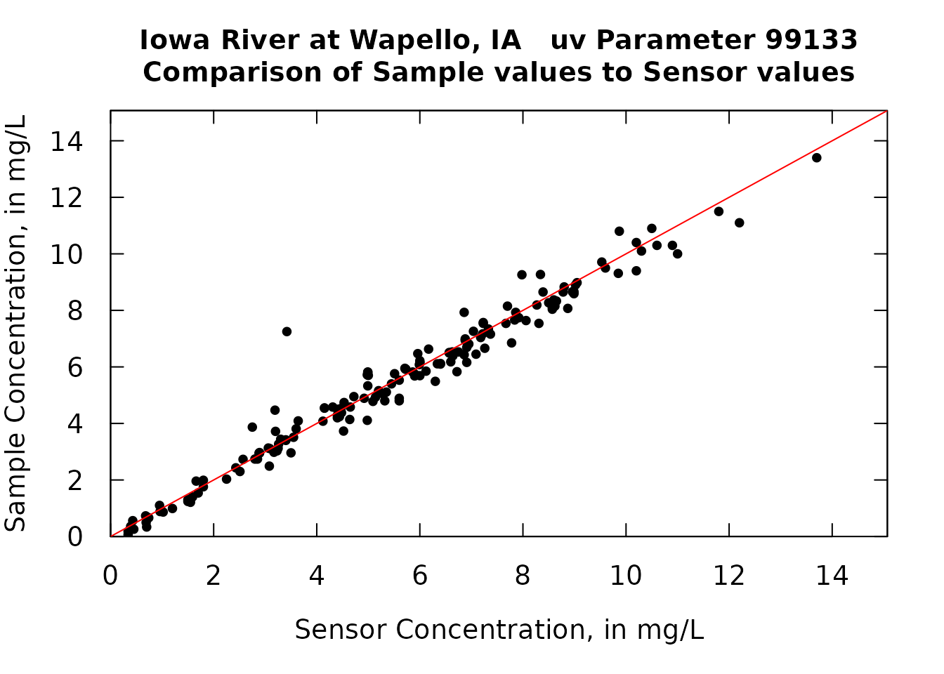
The plot shows that the relationship of the two variables is quite good, althought there does seem to be some bias. For example, for uv values greater than about 6 mg/L, the qw values tend to be a bit lower than the uv values.
Let’s do some exploratory data analysis to look at the consequences of just assuming that the uv values are a good approximation of the qw values.
resid <- Sam$ConcAve - Sam$uv
ymin <- min(resid)
ymax <- max(resid)
ylim <- c(ymin - 0.4, ymax + 0.4)
title <- paste0(staInfo$station_nm, "   uv Parameter ", pcode_uv,"\nError: Sample value minus Sensor value")
boxplot(resid, ylab = "Error, in mg/L", ylim = ylim, main = title)
abline(h = 0, col = "red")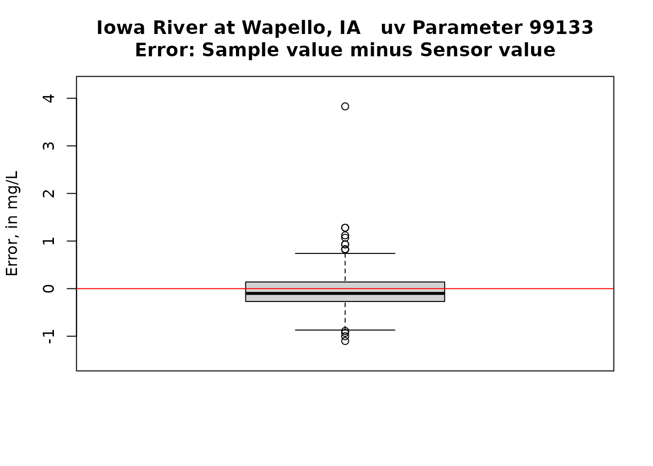
boxplot(resid~Sam$Month, ylab = "Error, in mg/L", ylim = ylim, main = title, xlab = "Month")
abline(h = 0, col = "red")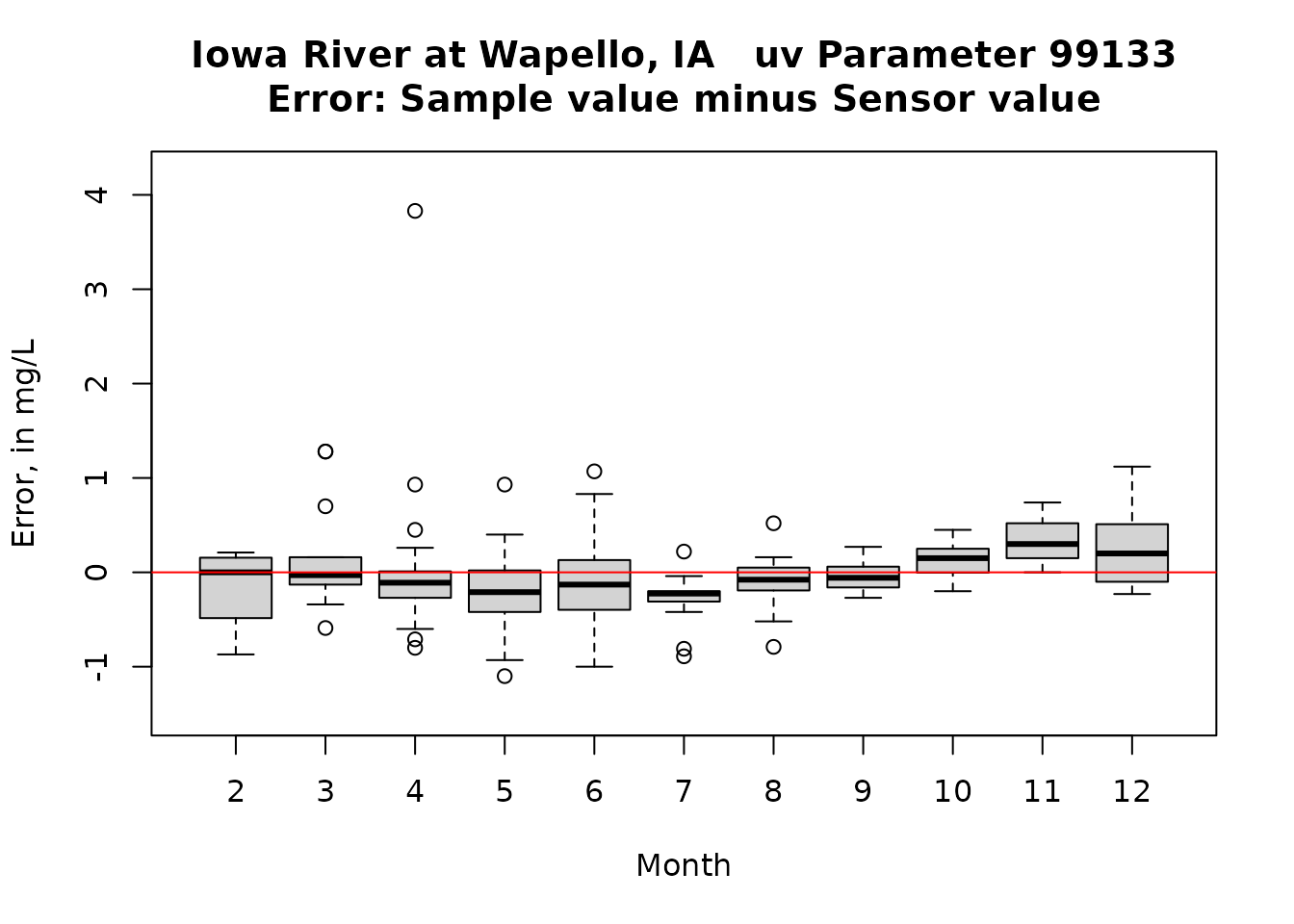
# note that there were no data pairs for January.  The Month indicator for the boxplot are the calendar months.
# thus 2 = February, 3 = March, etc.
title <- paste0(staInfo$station_nm, "   uv Parameter ", pcode_uv,"\nError as a function of sensor value")
xlim <- c(0, yMax * 1.1)
plot(Sam$uv, resid, pch = 19, cex = 0.6, ylim = ylim, ylab = "Error, in mg/L", main = title, xlim = xlim, xlab = "Sensor value, in mg/L")
axis(3, labels = FALSE)
axis(4, labels = FALSE)
abline(h = 0, col = "red")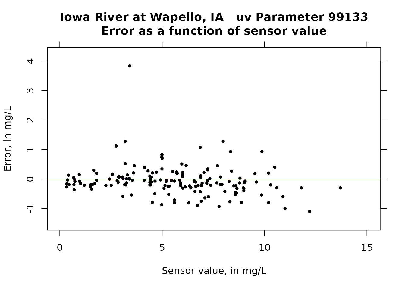
title <- paste0(staInfo$station_nm, "   uv Parameter ", pcode_uv,"\nError as a function DecYear")
xlim = c(2009, 2024)
plot(Sam$DecYear, resid, pch = 19, cex = 0.6, ylim = ylim, ylab = "Error, in mg/L", main = title, xlim = xlim, xlab = "")
axis(3, labels = FALSE)
axis(4, labels = FALSE)
abline(h = 0, col = "red")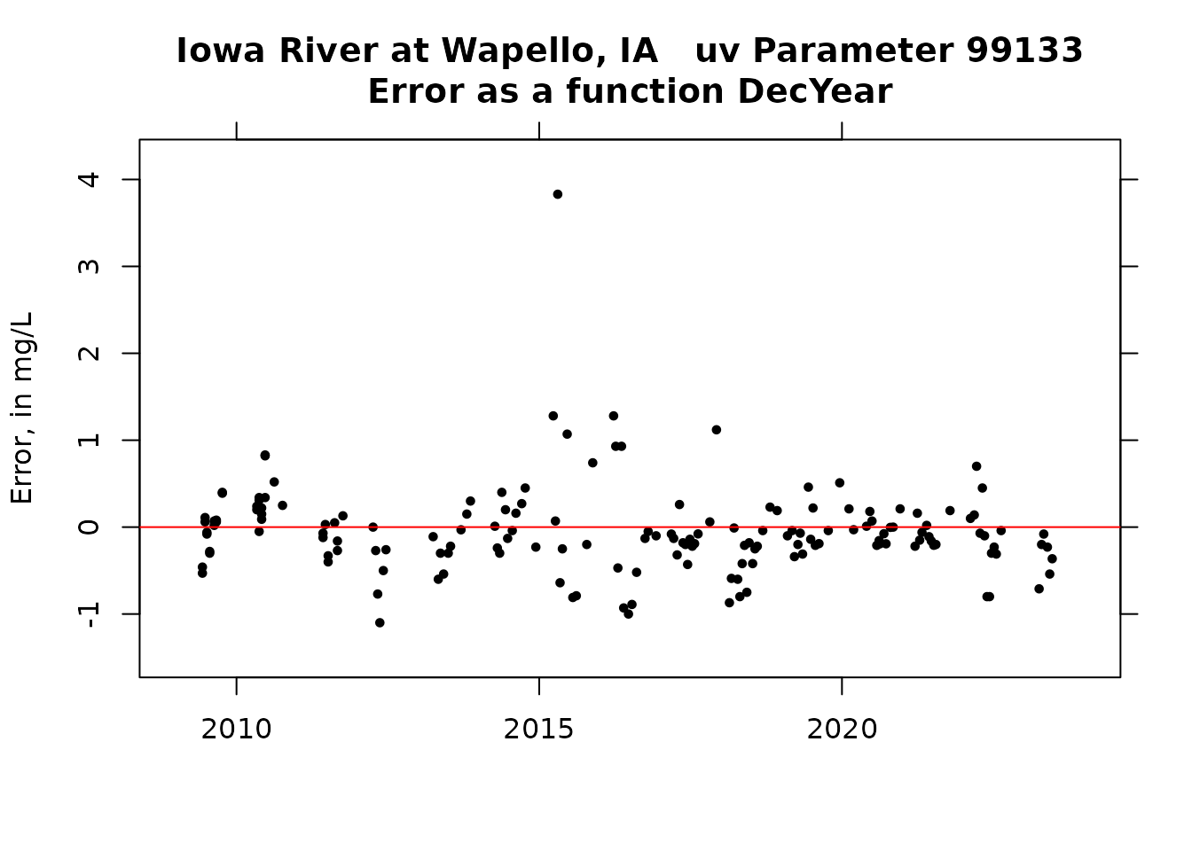
meanResid <- mean(resid)
medianResid <- median(resid)
stdDev <- sd(resid)
cat("\n Mean, Median, and Standard Deviation of the errors\n", meanResid, medianResid, stdDev)
##
## Mean, Median, and Standard Deviation of the errors
## -0.05012121 -0.1 0.5137924First impressions of the simple calibration
The errors are pretty nearly symmetrical and the bias is very small. Sensor values tend to slightly higher than sample values. There do seem to be some meaningful seasonal bias (some months consistently high and some consistantly low) and there is some drift in the relationship at the higher sensor values (Sample values are lower than sensor values).
Creating a calibration model
Let’s consider a multiple regression model to see if we can build a calibration equation that we can use. A more sophisticated approach might involve using smoothing concepts similar to WRTDS, but for this example, regression seems to work pretty well.
##
## Call:
## lm(formula = ConcAve ~ uv + DecYear + LogQ + SinDY + CosDY, data = Sam)
##
## Residuals:
##     Min      1Q  Median      3Q     Max
## -1.1542 -0.2318 -0.0184  0.1402  3.6797
##
## Coefficients:
##              Estimate Std. Error t value Pr(>|t|)
## (Intercept) 39.872649  19.547627   2.040  0.04303 *
## uv           0.947335   0.018385  51.528  < 2e-16 ***
## DecYear     -0.019985   0.009649  -2.071  0.03995 *
## LogQ         0.128755   0.063369   2.032  0.04384 *
## SinDY        0.059456   0.064093   0.928  0.35500
## CosDY        0.214767   0.072284   2.971  0.00343 **
## ---
## Signif. codes:  0 '***' 0.001 '**' 0.01 '*' 0.05 '.' 0.1 ' ' 1
##
## Residual standard error: 0.4872 on 159 degrees of freedom
## Multiple R-squared:  0.9702, Adjusted R-squared:  0.9693
## F-statistic:  1036 on 5 and 159 DF,  p-value: < 2.2e-16
The regression model is quite good. The R-squared value is 0.97. The overall regression equation is highly significant. Of course, most of the predictive power comes from the relationship between the uv values and the qw values. However, the coefficients on the other variables are all significant, so I would keep them in my calibration model. One might be tempted to say that SinDY should not be included in the model (the p value for it doesn’t turn out to be significant). However, we should keep it in the model because the other seasonal term (CosDY) is highly significant, and these two variables should always be treated as a pair, either both of them should be in the equation or both should be out (see page 346 in Statistical Methods in Water Resources, 2020 edition).
par(tck = 0.03, las = 1, xaxs = "i", yaxs = "i", cex.axis = 1.2, cex.lab = 1.2)
resid <- mod1$resid
ylim <- c(ymin - 0.4, ymax + 0.4)
title <- paste0(staInfo$station_nm, "   uv Parameter ", pcode_uv,"\nError: Sample value minus predicted value")
boxplot(resid, ylab = "Error, in mg/L", ylim = ylim, main = title)
abline(h = 0, col = "red")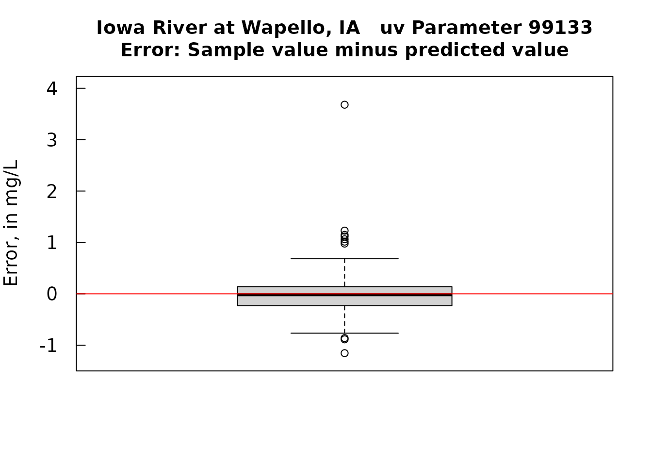
boxplot(resid~Sam$Month, ylab = "Error, in mg/L", ylim = ylim, main = title, xlab = "Month")
abline(h = 0, col = "red")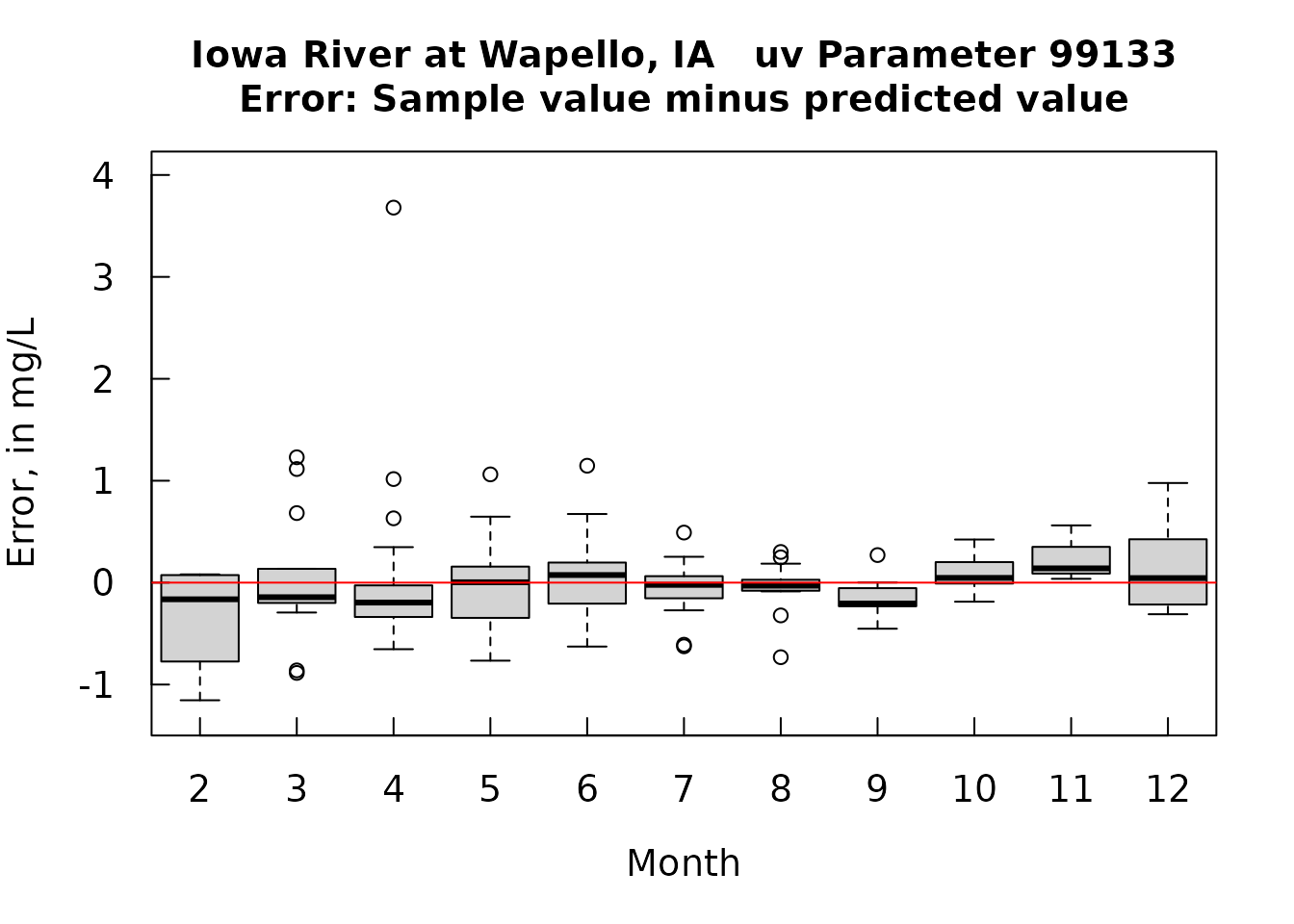
title <- paste0(staInfo$station_nm, "   uv Parameter ", pcode_uv,"\nError as a function of predicted value")
xlim <- c(0, yMax * 1.1)
plot(mod1$fit, resid, pch = 19, cex = 0.6, ylim = ylim, ylab = "Error, in mg/L", main = title, xlim = xlim, xlab = "Regression predicted value, in mg/L")
axis(3, labels = FALSE)
axis(4, labels = FALSE)
abline(h = 0, col = "red")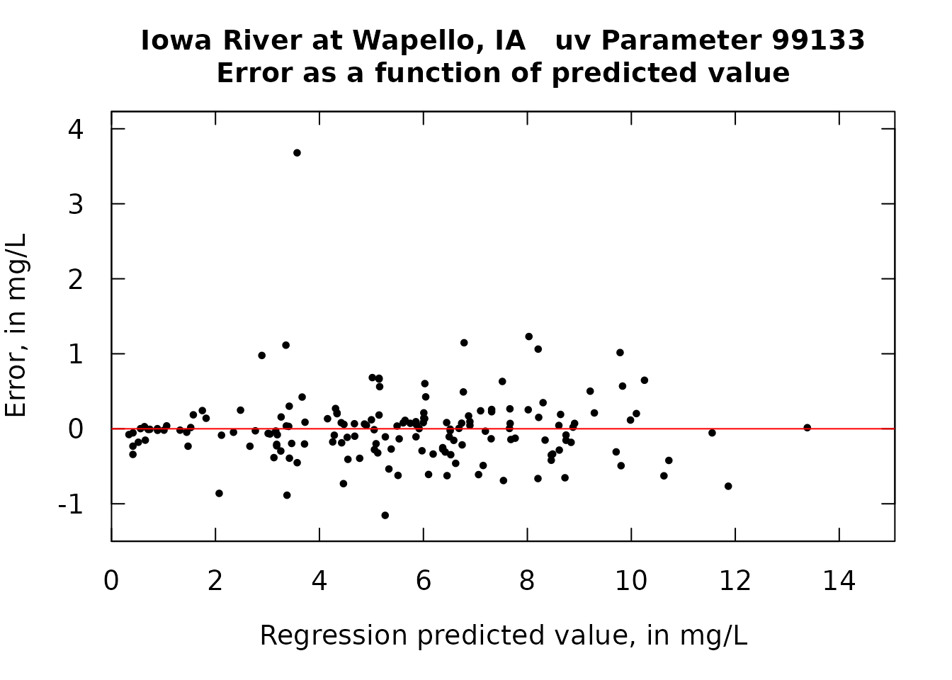
meanResid <- mean(resid)
medianResid <- median(resid)
stdDev <- sd(resid)
cat("\n Mean, Median, and Standard Deviation of the errors\n", meanResid, medianResid, stdDev)
##
## Mean, Median, and Standard Deviation of the errors
## -9.969732e-19 -0.01840193 0.4797555These preceeding plots indicate that the calibration model has done a pretty good job of producing unbiased estimates. The results do show some tendency towards being heteroscedastic so we might want to do this as a log-log regression, but for now I will leave the analysis at this point. My suggestion is that one use this calibration model with all of the sensor data to estimate nitrate concentrations. The results won’t be terribly different from just using the sensor value. But I would argue that these estimates will be slightly more accurate. The one issue of concern is that we do have sensor values in the full data set that go way outside the range of these data pairs. We are left with no choice but to do this extrapolation because we simply don’t have the sample values from the brief period when concentrations went up to 30 or more mg/L. There is some peril in doing that extrapolation but there is peril in not doing it. This is a place were experience at other sites may be useful in telling us if there are substantial bias issues at very high sensor values.
Using the calibration equation
What we will look at here is how we would apply the equation we just estimated in order to produce an unbiased estimate of concentration for every one of the unit value concentrations we have.
First we will need to make sure that we have a data frame of all the uv values, but since we are using have both a uv concentration value and a uv discharge (because these are both explanatory variables in the equation). We will eliminate from our uv record, those times for which one or both of these values is missing.
uv_data$Q <- uv_data$X_00060_00000 / 35.314667
uv_data$LQ <- log(uv_data$Q)
uv_data$SinDY <- sin(2 * pi * uv_data$DecYear)
uv_data$CosDY <- cos(2 * pi * uv_data$DecYear)
newdata <- data.frame(uv = uv_data$X_99133_00000, DecYear = uv_data$DecYear, LogQ = uv_data$LQ, SinDY = uv_data$SinDY, CosDY = uv_data$CosDY)
uv_data$pred <- predict(mod1, newdata = newdata, interval = "none")
plot(uv_data$X_99133_00000, uv_data$pred, pch = 19, cex = 0.1, xlab = "measured uv nitrate, in mg/L", ylab = "predicted uv nitrate, in mg/L", main = "Predicted nitrate values as a function of uv nitrate values")
abline(a = 0, b = 1, col = "red")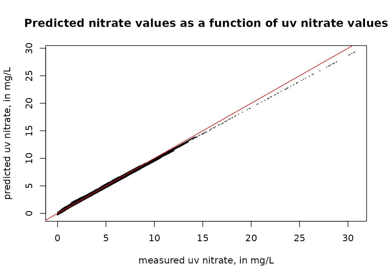
What we see here is that the predicted uv values (using the calibration equation) are very close to the measured uv value. But they do depart somewhat as we get to uv values above about 15 mg/L. Because we have no sample values in that range we have no meaningful way of checking the accuracy of that relationship.
It is notable that for moderate nitrate levels there is some variation in the values that we would estimate (as seen from the fact that the figure shows a cloud of points rather than a perfect straight line. Let’s see what that cloud looks like, by focusing in on a small segment of it, in this case uv values between 4.9 and 5.1 mg/L
xlim = c(4.9, 5.1)
ylim = c(4.5, 5.5)
plot(uv_data$X_99133_00000, uv_data$pred, pch = 19, cex = 0.1, xlab = "measured uv nitrate, in mg/L", ylab = "predicted uv nitrate, in mg/L", xlim = xlim, ylim = ylim, log = "xy", main = "Values of predicted nitrate\n over a narrow range of observed uv nitrate values")
abline(a = 0, b = 1, col = "red", lwd = 2)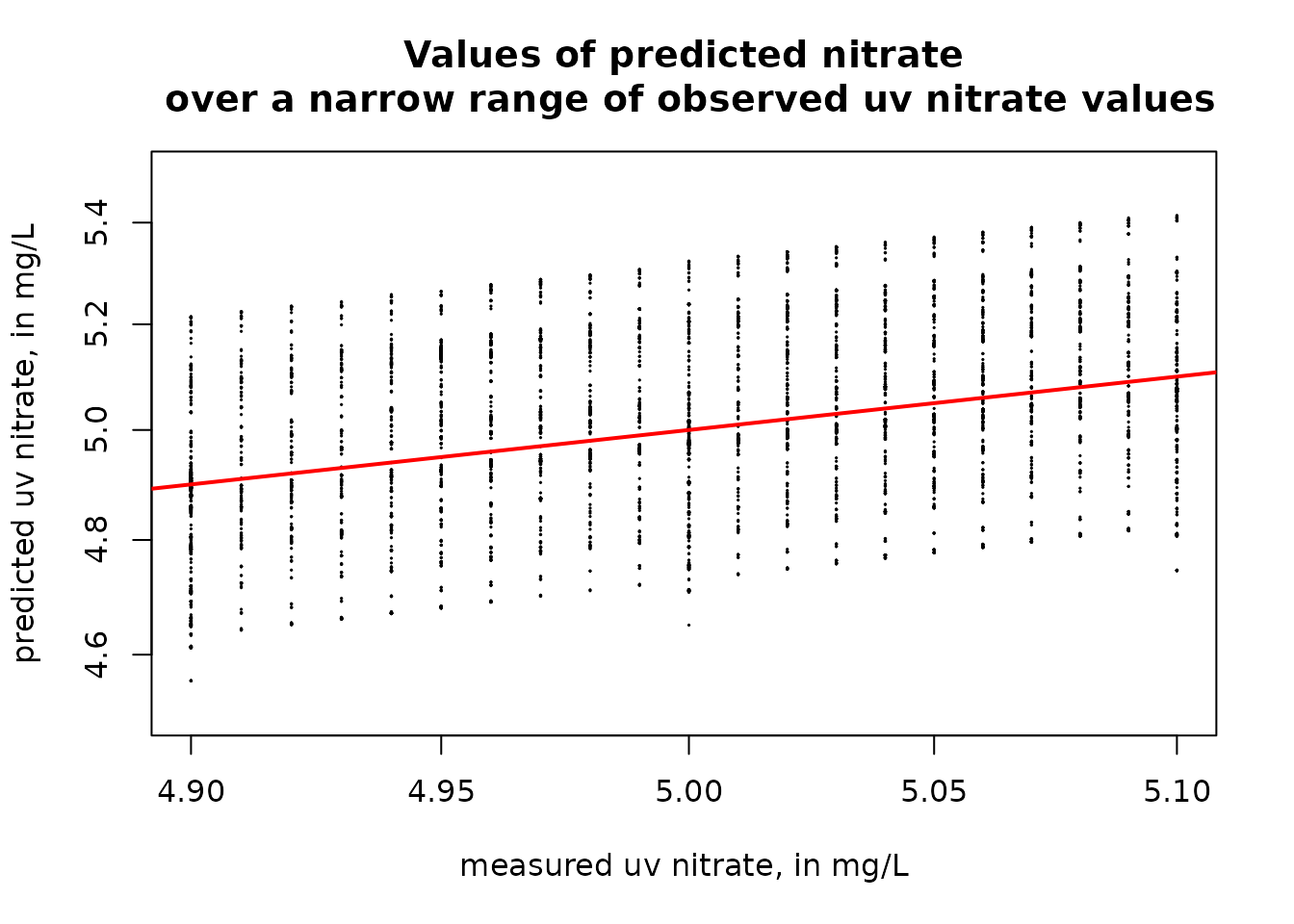
What we see here is that for any given uv value, the predictions can vary over a range of about 0.6 mg/L. This variation is driven by time of year, year, and discharge. This pattern indicates that these other variables do make a difference even though the primary driver in the calibration equation is the uv value. The observations on this graph show us that the uv data are reported with a precision of 0.01 mg/L, creating the series of vertical sets of points.
We can also look at the data as a time series showing the raw uv data and the calibration-adjusted value on the same graph. Here we do that for a portion of the year 2017.
xlim = c(2017.5, 2017.9)
ylim = c(0,12)
plot(uv_data$DecYear, uv_data$X_99133_00000, pch = 19, cex = 0.1, xlab = "", ylab = "nitrate concentration, in mg/L",
     xlim = xlim, ylim = ylim, main = "Raw uv nitrate data in black\nadjusted nitrate values in red")
points(uv_data$DecYear, uv_data$pred, pch = 19, cex = 0.05, col = "red")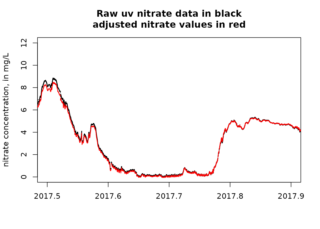
#
# here is another example time period
#
xlim = c(2022.3, 2022.7)
ylim = c(0,12)
plot(uv_data$DecYear, uv_data$X_99133_00000, pch = 19, cex = 0.1, xlab = "", ylab = "nitrate concentration, in mg/L",
     xlim = xlim, ylim = ylim, main = "Raw uv nitrate data in black\nadjusted nitrate values in red")
points(uv_data$DecYear, uv_data$pred, pch = 19, cex = 0.05, col = "red")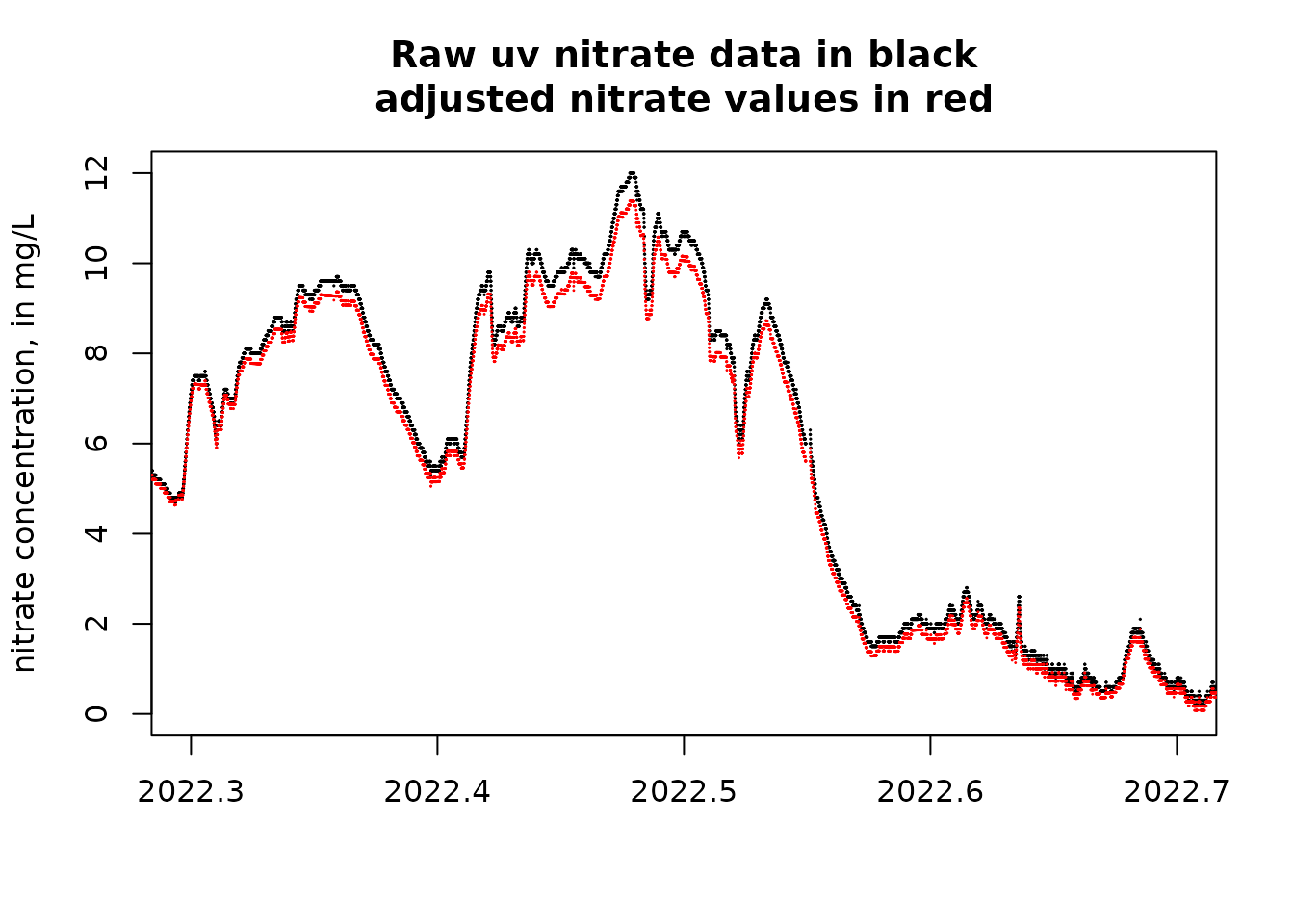
Concluding comments
These last two figures show us that the calibration process makes only a small amount of difference in this example, although it is notable that in the second of these last two figures, showing a time near the end of the record and at some rather high uv sensor values, there is a modest sized difference between the two values (calibrated versus uncalibrated).
I think that before decisions get made on the use of these types of calibration procedures there should be a lot more experimentation with data sets, similar to what is shown here for the Iowa River record. Also, there are probably other relationships between sensor values and sample values that are much less accurate than what we see here. My main point here is that when using these data for producing a product time series these kinds of steps should be taken.
In this particular case it is arguable whether the calibration process adds value to the data. The good it brings about is that it considers many factors in assessing the true value, but the potential cost of that is in the fact that many arbitrary choices are made in the form of the model and that there is a large amount of extrapolation required.
Next steps
These approaches need to be tried with a number of data sets.
-
They need to employ other sensors and other qw parameters. Some of options include things like.
Chloride based on specific conductance
Total phosphorus based on a combination of turbidity, pH, and other sensors
Rules need to be developed for completing a complete daily record combining these kinds of calibrated values for the days when there are uv data along with WRTDS-K values spanning those days when there are no uv data. There are a number of nuances invloved in this process that would need to be figured out, including whether the uv data are used in creating the WRTDS model which underlies the WRTDS-K estimates.
Finally, the question of producing flow-normalized concentration and flow-normalized fluxes, for trend evaluation. I have a work flow for that application and will probably add it to this vignette in the near future. There are several detailed method choices that would need to be evaluated before going forward with such approaches.
Robert Hirsch, February 7, 2024