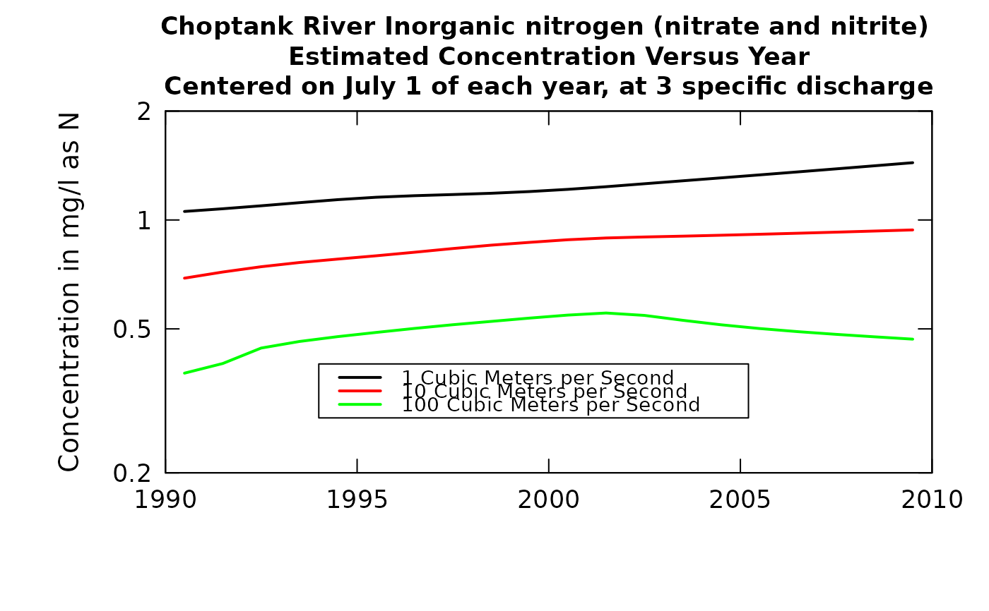
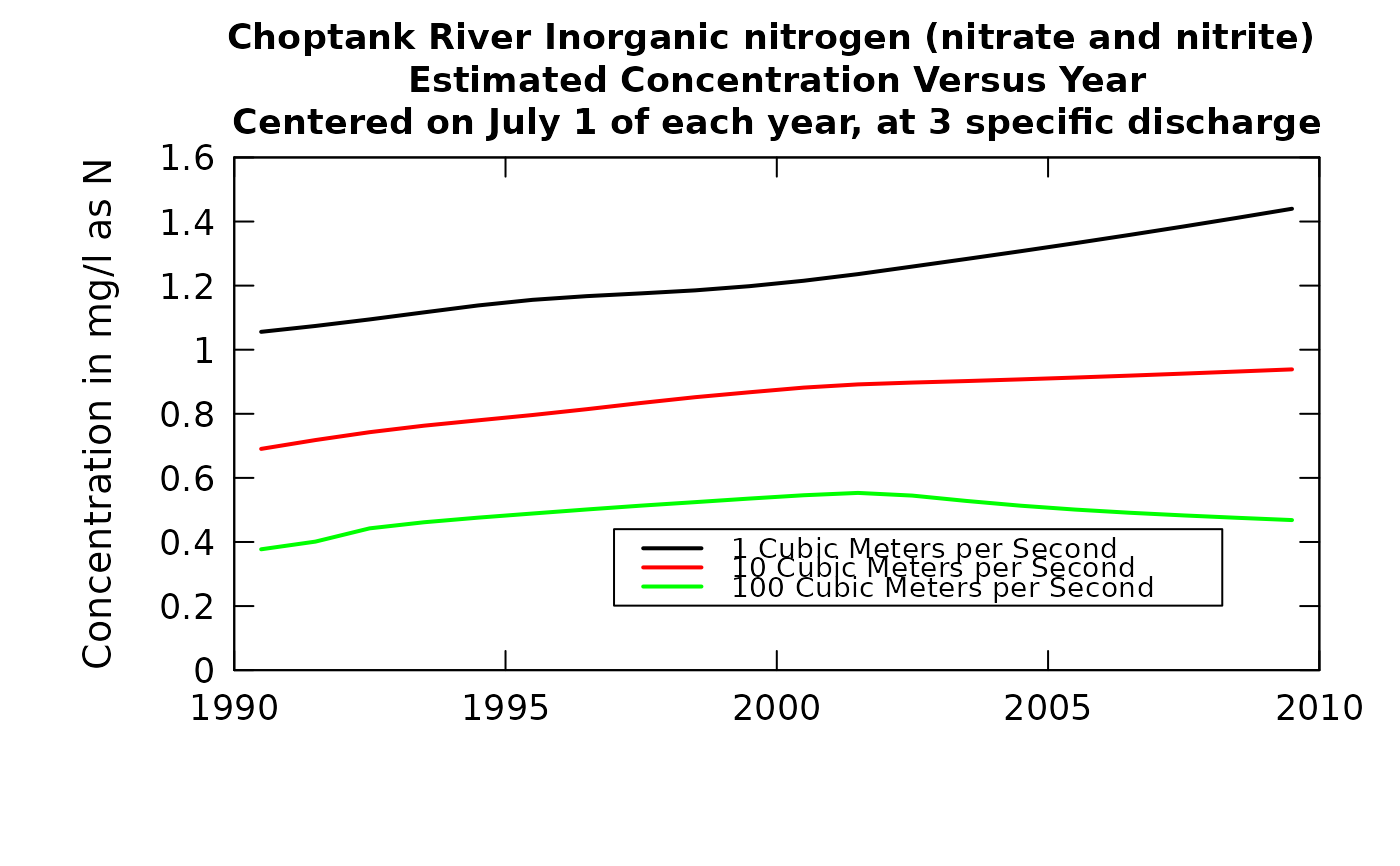
Plot up to three curves representing the concentration versus time relationship, each curve representing a different flow.

These plots show how the concentration-time relationship is changing over flow.

This plot can also help identify situations where the windowY may be too small. If there are substantial oscillations of some of the curves, then the windowY should be increased. Alternatively, windowY may be too large. This can be seen when the windowY is reduced (say to 4.0). A good choice of windowY would be a value just great enough to damp out oscillations in the curves.

Although there are a lot of optional arguments to this function, most are set to a logical default.

Data come from named list, which contains a Sample dataframe with the sample data and an INFO dataframe with metadata.

Usage

plotConcTimeSmooth(eList, q1, q2, q3, centerDate, yearStart, yearEnd,
  qUnit = 2, legendLeft = 0, legendTop = 0, concMax = NA,
  concMin = NA, bw = FALSE, printTitle = TRUE, colors = c("black",
  "red", "green"), printValues = FALSE, tinyPlot = FALSE, concLab = 1,
  monthLab = 1, minNumObs = 100, minNumUncen = 50, windowY = 10,
  windowQ = 2, windowS = 0.5, cex.main = 1.1, lwd = 2,
  printLegend = TRUE, cex.legend = 1.2, cex = 0.8, cex.axis = 1.1,
  customPar = FALSE, lineVal = c(1, 1, 1), logScale = FALSE,
  edgeAdjust = TRUE, usgsStyle = FALSE, ...)

Arguments

eList: named list with at least the Sample and INFO dataframes
q1: numeric This is the discharge value for the first curve to be shown on the plot. It is expressed in units specified by qUnit.
q2: numeric This is the discharge value for the second curve to be shown on the plot. It is expressed in units specified by qUnit. If you don't want a second curve then the argument must be q2=NA
q3: numeric This is the discharge value for the third curve to be shown on the plot. It is expressed in units specified by qUnit. If you don't want a third curve then the argument must be q3=NA
centerDate: character This is the time of year to be used as the center date for the smoothing. It is expressed as a month and day and must be in the form "mm-dd"
yearStart: numeric This is the starting year for the graph. The first value plotted for each curve will be at the first instance of centerDate in the year designated by yearStart.
yearEnd: numeric This is the end of the sequence of values plotted on the graph.The last value will be the last instance of centerDate prior to the start of yearEnd. (Note, the number of values plotted on each curve will be yearEnd-yearStart.)
qUnit: object of qUnit class. printqUnitCheatSheet, or numeric represented the short code, or character representing the descriptive name.
legendLeft: numeric which represents the left edge of the legend in the units of the plot.
legendTop: numeric which represents the top edge of the legend in the units of the plot.
concMax: numeric value for upper limit on concentration shown on the graph, default = NA (which causes the upper limit to be set automatically, based on the data)
concMin: numeric value for lower limit on concentration shown on the vertical log graph, default is NA (which causes the lower limit to be set automatically, based on the data). This value is ignored for linear scales, using 0 as the minimum value for the concentration axis.
bw: logical if TRUE graph is produced in black and white, default is FALSE (which means it will use color)
printTitle: logical variable if TRUE title is printed, if FALSE not printed
colors: color vector of lines on plot, see ?par 'Color Specification'. Defaults to c("black","red","green")
printValues: logical variable if TRUE the results shown on the graph are printed to the console and returned in a dataframe (this can be useful for quantifying the changes seen visually in the graph), default is FALSE (not printed)
tinyPlot: logical variable, if TRUE plot is designed to be plotted small, as a part of a multipart figure, default is FALSE
concLab: object of concUnit class, or numeric represented the short code, or character representing the descriptive name. By default, this argument sets concentration labels to use either Concentration or Conc (for tiny plots). Units are taken from the eList$INFO$param.units. To use any other words than "Concentration" see vignette(topic = "units", package = "EGRET").
monthLab: object of monthLabel class, or numeric represented the short code, or character representing the descriptive name.
minNumObs: numeric specifying the miniumum number of observations required to run the weighted regression, default is 100
minNumUncen: numeric specifying the minimum number of uncensored observations to run the weighted regression, default is 50
windowY: numeric specifying the half-window width in the time dimension, in units of years, default is 10
windowQ: numeric specifying the half-window width in the discharge dimension, units are natural log units, default is 2
windowS: numeric specifying the half-window with in the seasonal dimension, in units of years, default is 0.5
cex.main: magnification to be used for main titles relative to the current setting of cex
lwd: line width, a positive number, defaulting to 2
printLegend: logical if TRUE, legend is included
cex.legend: number magnification of legend
cex: numerical value giving the amount by which plotting symbols should be magnified
cex.axis: magnification to be used for axis annotation relative to the current setting of cex
customPar: logical defaults to FALSE. If TRUE, par() should be set by user before calling this function (for example, adjusting margins with par(mar=c(5,5,5,5))). If customPar FALSE, EGRET chooses the best margins depending on tinyPlot.
lineVal: vector of line types. Defaults to c(1,1,1) which is a solid line for each line. Options: 0=blank, 1=solid (default), 2=dashed, 3=dotted, 4=dotdash, 5=longdash, 6=twodash
logScale: logical whether or not to use a log scale in the y axis.
edgeAdjust: logical specifying whether to use the modified method for calculating the windows at the edge of the record. The modified method tends to reduce curvature near the start and end of record. Default is TRUE.
usgsStyle: logical option to use USGS style guidelines. Setting this option to TRUE does NOT guarantee USGS compliance. It will only change automatically generated labels
...: arbitrary functions sent to the generic plotting function. See ?par for details on possible parameters

Examples

q1 <- 1
q2 <- 10
q3 <- 100
centerDate <- "07-01"
yearStart <- 1990
yearEnd <- 2010
eList <- Choptank_eList
plotConcTimeSmooth(eList, q1, q2,q3, centerDate, 
                   yearStart, yearEnd, legendLeft = 1997, 
                   legendTop = 0.44, cex.legend = 0.9)

plotConcTimeSmooth(eList, q1, q2,q3, centerDate, yearStart, 
                   yearEnd, logScale = TRUE, legendLeft = 1994, 
                   legendTop = 0.4, cex.legend = 0.9)

Plot up to three curves representing the concentration versus time relationship, each curve representing a different flow.

Usage

Arguments

See also

Examples