Plot monthly trend result from runPairs — plotMonthTrend • EGRET

Plot monthly trend result from runPairs. The change in concentration or flux is calculated from the runPairs function. This plotting function shows an arrow for each month. If the trend from year1 to year2 was increasing, the arrow is red and pointing up. If the trend was decreasing, the arrow is black and pointing down.

Usage

plotMonthTrend(pairResults, yMax = NA, arrowFactor = 0.75, flux = TRUE,
  printTitle = TRUE, concLab = 1, monthLab = 1)

Arguments

pairResults: results from runPairs.
yMax: numeric. Upper limit for plot. Default is NA, which will use the maximum of the data.
arrowFactor: numeric. Scaling factor for the size of the arrows. The arrows are automatically scaled to the overall trend. This scaling factor helps adjust how big/small they are.
flux: logical. TRUE is flux, FALSE is concentration. Default is TRUE.
printTitle: logical variable if TRUE title is printed, if FALSE title is not printed (this is best for a multi-plot figure)
concLab: object of concUnit class, or numeric represented the short code, or character representing the descriptive name. By default, this argument sets concentration labels to use either Concentration or Conc (for tiny plots). Units are taken from the eList$INFO$param.units. To use any other words than "Concentration" see vignette(topic = "units", package = "EGRET").
monthLab: object of monthLabel class, or numeric represented the short code, or character representing the descriptive name.

Value

Base R plot of monthly trends

Details

The flux values for each month are flow normalized monthly watershed yields expressed as kg/month/km^2. The concentrations are the mean flow normalized concentration, expressed in whatever concentration units the raw data are expressed as (typically mg/L).

Examples


eList <- Choptank_eList
year1 <- 1985
year2 <- 2010

# \donttest{

pairOut_1 <- runPairs(eList, year1, year2, windowSide = 0)
#> Sample1 has 606 Samples and 605 are uncensored
#> Sample2 has 606 Samples and 605 are uncensored
#> minNumObs has been set to 100 minNumUncen has been set to 50
#> Sample1 has 606 Samples and 605 are uncensored
#> Sample2 has 606 Samples and 605 are uncensored
#> minNumObs has been set to 100 minNumUncen has been set to 50
#> 
#>    Choptank River 
#>    Inorganic nitrogen (nitrate and nitrite)
#>    Water Year 
#> 
#>  Change estimates  2010  minus  1985 
#> 
#>  For concentration: total change is  0.429 mg/L
#>  expressed as Percent Change is  +42.27 %
#> 
#>  Concentration v. Q Trend Component  +42.27 % 
#>        Q Trend Component              0 %  
#> 
#> 
#>  For flux: total change is  0.0342 million kg/year
#>  expressed as Percent Change is  +29.44 %
#> 
#>  Concentration v. Q Trend Component  +29.44 % 
#>        Q Trend Component              0 %  
#> 
#>      TotalChange  CQTC QTC  x10  x11  x20  x22
#> Conc       0.429 0.429   0 1.01 1.01 1.44 1.44
#> Flux       0.034 0.034   0 0.12 0.12 0.15 0.15

plotMonthTrend(pairOut_1)

plotMonthTrend(pairOut_1, flux = FALSE)


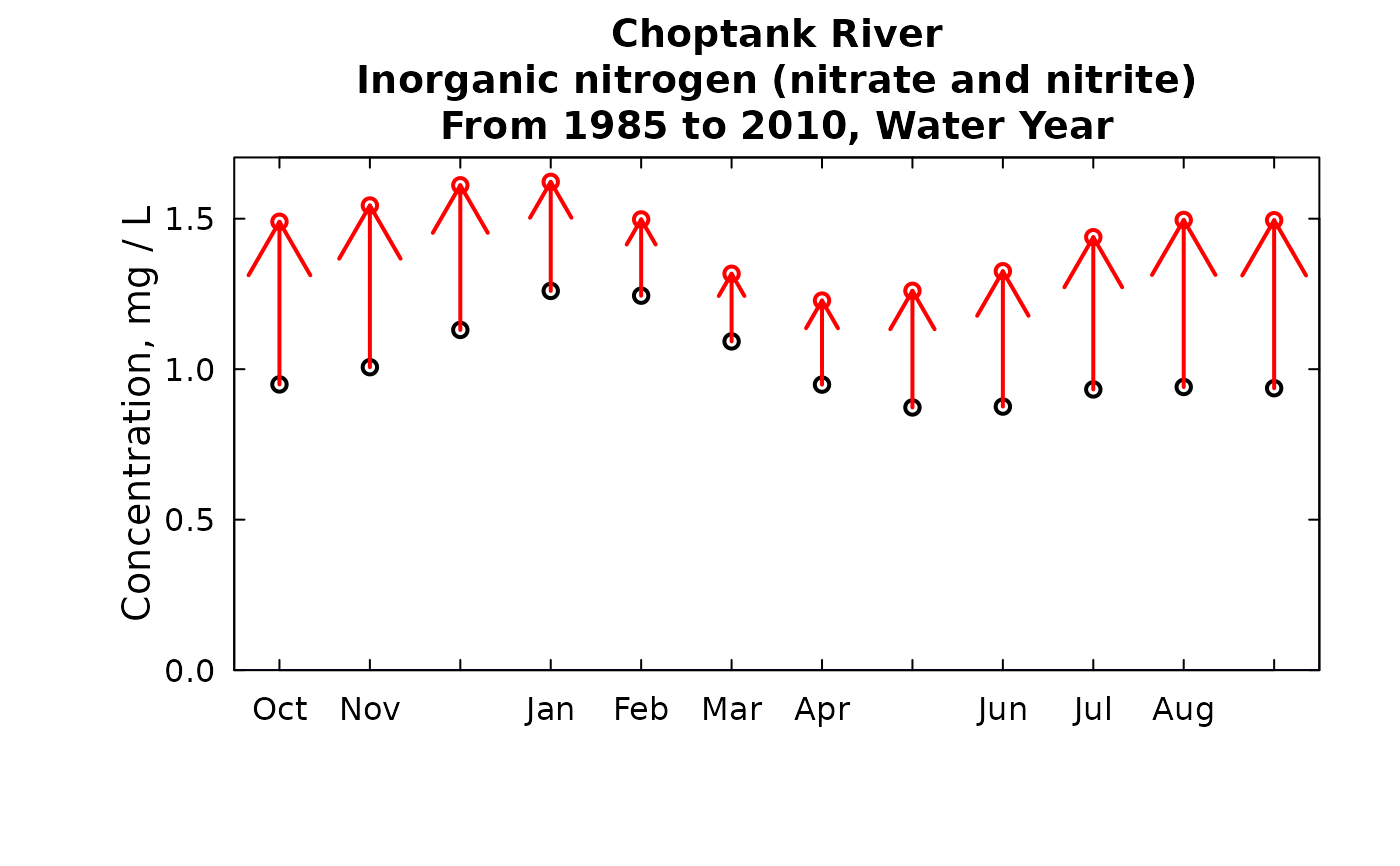eList <- setPA(eList, paStart = 12, paLong = 3)
pairOut_2 <- runPairs(eList, year1, year2, windowSide = 0)
#> Sample1 has 606 Samples and 605 are uncensored
#> Sample2 has 606 Samples and 605 are uncensored
#> minNumObs has been set to 100 minNumUncen has been set to 50
#> Sample1 has 606 Samples and 605 are uncensored
#> Sample2 has 606 Samples and 605 are uncensored
#> minNumObs has been set to 100 minNumUncen has been set to 50
#> 
#>    Choptank River 
#>    Inorganic nitrogen (nitrate and nitrite)
#>    Season Consisting of Dec Jan Feb 
#> 
#>  Change estimates  2010  minus  1985 
#> 
#>  For concentration: total change is  0.369 mg/L
#>  expressed as Percent Change is  +30.50 %
#> 
#>  Concentration v. Q Trend Component  +30.50 % 
#>        Q Trend Component              0 %  
#> 
#> 
#>  For flux: total change is  0.0403 million kg/year
#>  expressed as Percent Change is  +22.68 %
#> 
#>  Concentration v. Q Trend Component  +22.68 % 
#>        Q Trend Component              0 %  
#> 
#>      TotalChange CQTC QTC  x10  x11  x20  x22
#> Conc        0.37 0.37   0 1.21 1.21 1.58 1.58
#> Flux        0.04 0.04   0 0.18 0.18 0.22 0.22

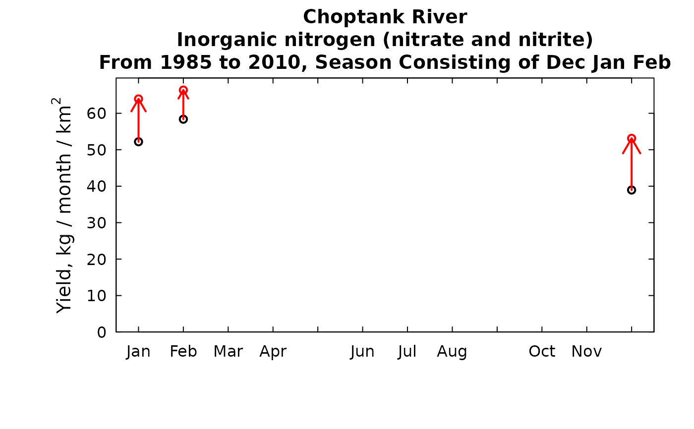
plotMonthTrend(pairOut_2)


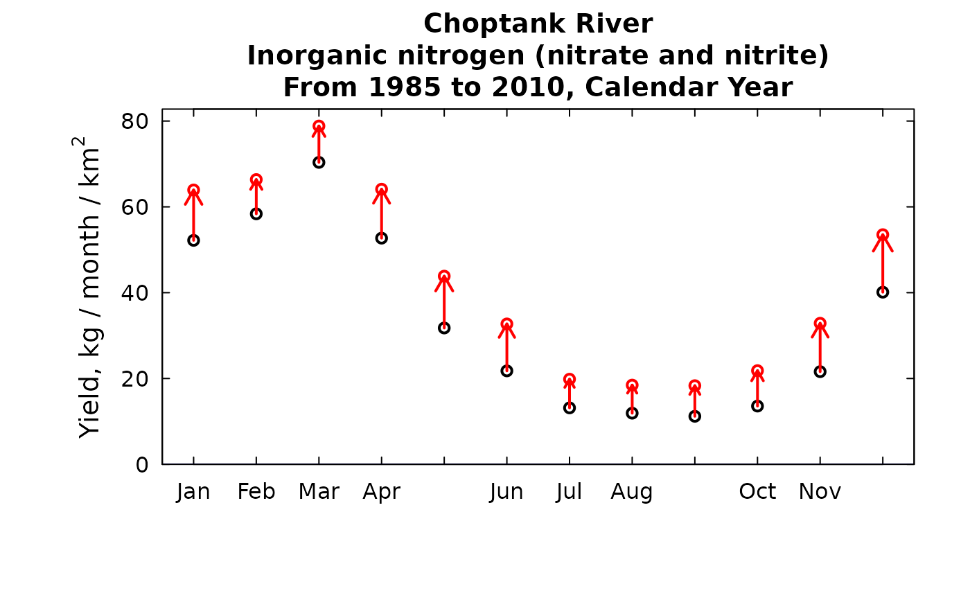
eList <- setPA(eList, paStart = 1, paLong = 12)
pairOut_3 <- runPairs(eList, year1, year2, windowSide = 0)
#> Sample1 has 606 Samples and 605 are uncensored
#> Sample2 has 606 Samples and 605 are uncensored
#> minNumObs has been set to 100 minNumUncen has been set to 50
#> Sample1 has 606 Samples and 605 are uncensored
#> Sample2 has 606 Samples and 605 are uncensored
#> minNumObs has been set to 100 minNumUncen has been set to 50
#> 
#>    Choptank River 
#>    Inorganic nitrogen (nitrate and nitrite)
#>    Calendar Year 
#> 
#>  Change estimates  2010  minus  1985 
#> 
#>  For concentration: total change is  0.433 mg/L
#>  expressed as Percent Change is  +42.46 %
#> 
#>  Concentration v. Q Trend Component  +42.46 % 
#>        Q Trend Component              0 %  
#> 
#> 
#>  For flux: total change is  0.034 million kg/year
#>  expressed as Percent Change is  +29.09 %
#> 
#>  Concentration v. Q Trend Component  +29.09 % 
#>        Q Trend Component              0 %  
#> 
#>      TotalChange  CQTC QTC  x10  x11  x20  x22
#> Conc       0.433 0.433   0 1.02 1.02 1.45 1.45
#> Flux       0.034 0.034   0 0.12 0.12 0.15 0.15

plotMonthTrend(pairOut_3)


# }