Guide to EGRETci 2.0 enhancements
Robert M. Hirsch and Laura De Cicco
2018-06-18
Source:vignettes/Enhancements.Rmd
Enhancements.RmdIntroduction
This vignette documents a set of enhancements of the
EGRETci software package. EGRET is
“Exploration and Graphics for RivEr Trend” which has been developed my
Robert M. Hirsch and Laura DeCicco of the U.S. Geological Survey. The
EGRETci package contains functions that can be used to
evaluate the uncertainty associated with results generated by the
EGRET code. This document, on the EGRETci 2.0
enhancements assumes that the reader already has a good understanding of
WRTDS (Weighted Regressions on Time Discharge and Season), and the
EGRET 2.0 package and the EGRET 3.0
enhancements (“Guide to EGRET 3.0 enhancements”) as well as the
documentation “Introduction to EGRET Confidence Intervals”“). The two
releases EGRET 3.0 and EGRETci 2.0 are tightly
linked in terms of naming conventions and the sharing of various objects
between them. Brief reference is made to these EGRETci functions in the
documentation of the EGRET 3.0 enhancements.
The releases of EGRET 3.0 add some new flexibility to the WRTDS method. The flexibility that the new version provides are of two kinds. One is an ability to partition the sample data into two periods, one before and one after, a change that happened in the watershed that we believe to have had an important, sudden, but lasting impact on water quality. The other is the ability to relax the assumption of stationarity of streamflow in the flow normalization process. As shorthand we refer to the first of these enhancements as the “wall”, and the second as “Generalized Flow Normalization.” These are discussed in detail in “Guide to EGRET 3.0 enhancements” and are not repeated here.
This document discusses the motivations and general concepts behind these enhancements, and then move to instructions for implementation. It is assumed that the reader already has a good working knowledge of WRTDS, EGRET and EGRETci. Hirsch, Moyer and Archfield, 2010, Hirsch and DeCicco, 2015, Hirsch, Archfield and DeCicco, 2015 and the Introduction to the EGRET package, and Introduction to EGRET Confidence Intervals.
EGRETci 2.0 is designed so that it will produce
exactly the same outputs as EGRETci 1.0 version did
using the same set of commands that would have been used with one
notable exception. Previous versions of EGRETci did not
require a “startSeed” argument when running the confidence intervals in
parallel. The reason for the change is to assure that we can now
reproduce all bootstrapping calculations. It is important to adjust any
parallel code to include that argument as follows (specifically the
“startSeed = n” argument):
nCores <- detectCores() - coreOut
cl <- makeCluster(nCores)
registerDoParallel(cl)
repAnnual <- foreach(n = 1:nBoot,.packages=c('EGRETci')) %dopar% {
   annualResults <- bootAnnual(eList,
                               blockLength,
                               startSeed = n)
}
stopCluster(cl)
Problem set up
There are three distinct types of problem set-ups that are possible in the new formulation and each of them has its own distinct workflow and outputs. They are known as Pairs, Series, and Groups. What do these terms mean here? Pairs is for the comparison of any two years in the study period, Series is to describe the entire study period to produce graphs of the change as a function of time, Groups is for the comparison of any two groups of contiguous years. The appropriate use of each of these three set-ups is described in detail in the “Guide to EGRET 3.0 enhancements.”
runPairsBoot: The bootstrap uncertainty analysis for runPairs results
The function that does the uncertainty analysis for determining the
change between any pair of years is called
runPairsBoot. It is very similar to the
wBT function that runs the WRTDS Bootstrap Test in
EGRETci 1.0. It differs from wBT in that
it runs a specific number of bootstrap replicates, unlike the
wBT approach that will stop running replicates based on
the status of the test statistics along the way.
The call to runPairsBoot is very simple, because it gets virtually all of the information about how the analysis is to be set up from information in the attributes of pairResults. The only arguments that are required are the eList and pairResults and three more arguments specifically related to the bootstrap process. These are described here:
nBoot This is the number of bootstrap replicates to run. It has a default value of 100. A value of 100 should give rough approximation of the correct likelihood of the trend direction. For example, if the bootstrap results were upwards trends in 98 of 100 replicates, then we could say that we have about 95% confidence that the true likelihood that the trend is upwards is between 0.945 and 0.998 (rather strong evidence of an upwards trend). For purposes of a published study going to nBoot = 500 may be appropriate. For example if we had 490 upwards trends out of 500 replicates we could say with 95% confidence that the likelihood that the true trend is upwards is between 0.966 and 0.991. To see if it is even worthwhile to do a large number of replicates one could use a very small number of replicates, say nBoot = 10 and if there is a fairly even mix of increases and decreases we can dispense with the high number of replicates and simply conclude that it is about as likely up as it is down. In a few cases some of the bootstrap replicates have results that do not converge and they generate an error message but no results for that replicate. To deal with that, the function is designed to run more replicates than nBoot but to quit when it reaches nBoot
startSeed This is the seed for the random number generator, which is used to create the random bootstrap replicates of the data. It has a default value but any integer will work. Knowing the startSeed value is vital to reproducing the results. If a different value of startSeed is used in a later run it will produce slightly different results, but with nBoot of 200 or more these differences should be trivially small.
blockLength This is the block length for the block bootstrap resampling (see Hirsch, Archfield and DeCicco, 2015 for an explanation). This argument has a default of 200 so it shouldn’t need to be specified.
Here we will run a trivially small example of
runPairsBoot based on the problem set up in the second
example of runPairs in the EGRET 3.0 enhancements User
Guide.
library(EGRET)
library(EGRETci)
eList <- Choptank_eList
pairResults2 <- runPairs(eList, year1 = 1985, year2 = 2010,
                         windowSide = 7, flowBreak = TRUE,
                         Q1EndDate = "1995-05-31", wall = TRUE,
                         sample1EndDate = "1995-05-31",
                         QStartDate = "1979-10-01",
                         QEndDate = "2010-09-30",
                         paStart = 4, paLong = 5)
bootPairOut2 <- runPairsBoot(eList,
                             pairResults2,
                             nBoot = 10)
 iBoot, xConc and xFlux 1 0.4048814 0.03866322
 iBoot, xConc and xFlux 2 0.4186308 0.04813132
 iBoot, xConc and xFlux 3 0.4114679 0.04757094
 iBoot, xConc and xFlux 4 0.4314246 0.04415677
 iBoot, xConc and xFlux 5 0.3456514 0.03323089
 iBoot, xConc and xFlux 6 0.4639338 0.04792485
 iBoot, xConc and xFlux 7 0.3480087 0.03212271
 iBoot, xConc and xFlux 8 0.3694464 0.03815445
 iBoot, xConc and xFlux 9 0.3502027 0.04509857
 iBoot, xConc and xFlux 10 0.4180412 0.04559656
   Choptank River
   Inorganic nitrogen (nitrate and nitrite)
   Season Consisting of Apr May Jun Jul Aug


 Change estimates are for  2010  minus  1985
 Sample data set was partitioned with a wall at  1995-05-31


Should we reject Ho that Flow Normalized Concentration Trend = 0 ? Reject Ho
 best estimate of change in concentration is   0.412 mg/L
  Lower and Upper 90% CIs    0.346    0.464
 also 95% CIs    0.346    0.464
 and 50% CIs    0.350    0.422
 approximate two-sided p-value for Conc      0.18
* Note p-value should be considered to be < stated value
 Likelihood that Flow Normalized Concentration is trending up = 0.955  is trending down = 0.0455

Should we reject Ho that Flow Normalized Flux Trend = 0 ? Reject Ho
 best estimate of change in flux is   0.0456 10^6 kg/year
  Lower and Upper 90% CIs   0.0321   0.0481
 also 95% CIs   0.0321   0.0481
 and 50% CIs   0.0369   0.0477
 approximate two-sided p-value for Flux      0.18
* Note p-value should be considered to be < stated value
 Likelihood that Flow Normalized Flux is trending up = 0.955  is trending down = 0.0455

 Upward trend in concentration is highly likely
 Upward trend in flux is highly likely
 Downward trend in concentration is highly unlikely
 Downward trend in flux is highly unlikely
The output is pretty self-explanatory and the latter part of it is identical to the summary information provided by wBT.
The object returned by runPairsBoot is virtually the same as the eBoot object returned by wBT. It contains the data frame called bootOut which contains all the results of the test that are shown in the console. One new feature here is bootOut$nBootGood. Because there is a small chance that the bootstrap results will contain a small number of iterations that fail to complete it may end up with a number of valid replicates that is less than nBoot. The number of usable replicates is nBootGood. The other parts of the returned object are the same as those returned from wBT.
One of the outputs we can use to describe the results of the test is
the histogram of percentage changes. These can be done with the
plotHistogramTrend function just as they have been in
the EGRETci 1.0.3 software. The only difference in the call
to the function is that we don’t use caseSetUp in
runPairs so that argument is set to caseSetUp =
NA.
To call this function for a runPairsBoot result would look like this:
plotHistogramTrend(eList, eBoot, caseSetUp = NA,
                   flux = TRUE, xMin = NA, xMax = NA,
                   xStep = NA, printTitle = TRUE,
                   cex.main = 1.1, cex.axis = 1.1,
                   cex.lab = 1.1, col.fill = "grey", ...)
The only two arguments required are eList, and eBoot which represents the output from runPairsBoot.
Here are the calls to plotHistogramTrend first for flux, and then for concentration. [We have substituted in a set of runPairsBoot outputs for which nBoot = 100 rather than using the one shown above.]
bootPairOut2 <- runPairsBoot(eList, pairResults2, nBoot = 100)Here are the calls to plotHistogramTrend first for flux, and then for concentration.
plotHistogramTrend(eList,bootPairOut2, caseSetUp = NA)
plotHistogramTrend(eList,bootPairOut2, caseSetUp = NA, flux = FALSE)
So, what the results clearly show us is that flux has clearly increased and probably by a magnitude of a few hundred percent and concentration has clearly increased probably by an amount between about 100 % to 200 %.
The bootstrap uncertainty analysis for runSeries
The purpose of Series analysis is to create a time series of flow-normalized concentrations and flow-normalized flux values. The function that does this is runSeries in the EGRET package.
In the case of runSeries we can do uncertainty analysis which provides us with confidence intervals around the flow normalized time series that we estimated from running the runSeries function. In this case we actually use the same functions that were used in EGRETci 1.0.3, but they have been modified here to accommodate all of the flexible features of runSeries (but they run exactly as they did before if they were just working off of results from modelEstimation).
This is how it is called:
CIAnnualResults <- ciCalculations(eList,
                                  startSeed = 494817,
                                  verbose = TRUE, ...)
The eList that is passed to the function should be a version of eList that has already been run through runSeries. So, for the example run shown above the eList argument would be eListOut. That version contains all the estimated values as well as all of the arguments that were used in the computation (related to the wall and flowBreak etc.). There is no need to specify startSeed, the default will be fine (unless one wants to explore how the results might change in another run of the function). To avoid seeing all the progress indicators on the screen one can set verbose = FALSE, but it may be desirable just to see that the job is continuing to run by setting verbose = TRUE. It can take a considerable amount of computer time.
The ... in the call specifically relate to some other
bootstrap-related parameters that the user might wish to set. They can
be left out of the call, and the program with interactively request the
information, or they can be set directly in the call. We will set up to
run the job specifying them without the interactive part (as would be
done in a batch implementation).
We will run the bootstrap analysis here. We will use the output of the last run of runSeries example in the EGRET enhancement vignette.
eList <- Choptank_eList
eListOut <- runSeries(eList, windowSide = 7, verbose = FALSE)
CIAnnualResults <- ciCalculations(eListOut,
                                  verbose = FALSE,
                                  nBoot = 100,
                                  blockLength = 200,
                                  widthCI = 90)
CIAnnualResults <- ciCalculations(eListOut,
                                  verbose = FALSE,
                                  nBoot = 100,
                                  blockLength = 200,
                                  widthCI = 90)
nBoot is the number of bootstrap replicates to be run. A result that is suitable for publication should probably have nBoot at least 100 and preferably 200. blockLength is typically set to 200. widthCI is the width of the confidence interval. If widthCI = 90 that means that the confidence intervals that will be drawn are the 5th and 95th percentiles.
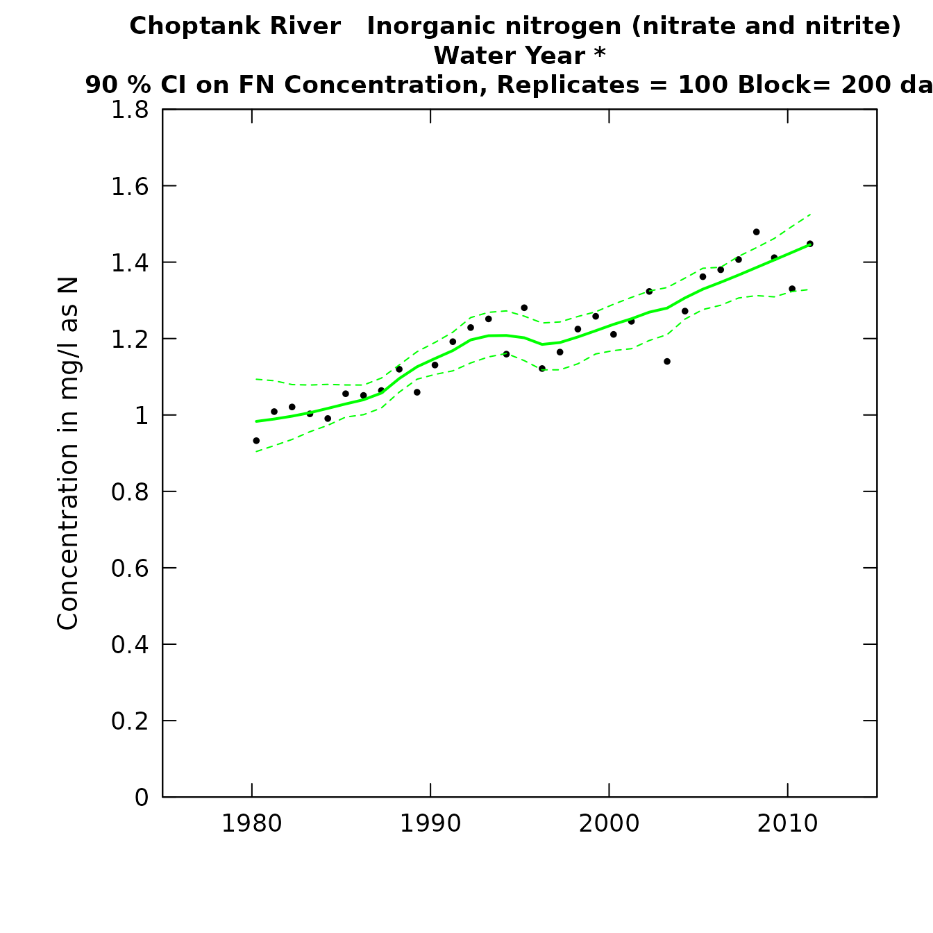
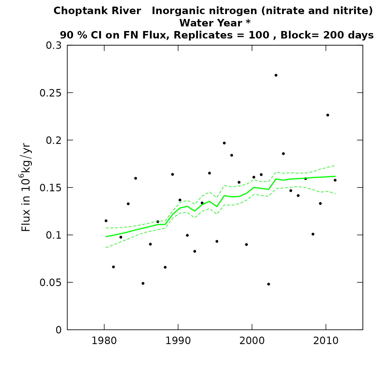
We can visualize the results by using the plotConcHistBoot and plotFluxHistBoot functions (which were a part of the EGRETci 1.0.3 code). Running them with results from runSeries requires that we use the eList that is produced by the runSeries function. So, following the results we saw from runSeries we would obtain the confidence interval plots as follows. (Note that there are several other arguments to these functions that are the same as those used in plotConcHist and plotFluxHist).
plotConcHistBoot(eListOut, CIAnnualResults)
plotFluxHistBoot(eListOut, CIAnnualResults) Looking at the output, particularly for plotFluxHistBoot, suggests that
the windowSide argument is probably too short. The plot is simply too
jagged. A better choice would probably have been to set windowSide = 11.
We have included this example here to show the problem of having
windowSide be too small. The general conclusions about the overall
increase over the more than 30 year record would remain the same and the
width of the confidence intervals wouldn’t change much if a better
windowSide argument had been used.
runGroupsBoot: The bootstrap uncertainty analysis for runGroups results
The function that does the uncertainty analysis for determining the change between two groups of years is called runGroupsBoot. The process is virtually identical to what is used for runPairsBoot, so much of the detail will be left out of this discussion. The call to runGroupsBoot is very simple, because it gets virtually all of the information about how the analysis is to be set up from information in the attributes of groupResults. The only arguments that are required are the eList and groupResults and three more arguments specifically related to the bootstrap process:
nBoot This is the number of bootstrap replicates to run. It has a default value of 100. In a few cases some of the bootstrap replicates have results that do not converge and they generate an error message but no results for that replicate. To deal with that the function is designed to run more replicates than nBoot but to quit when it reaches nBoot
startSeed This is the seed for the random number generator, which is used to create the random bootstrap resamples of the data. It has a default value but any integer will work.
blockLength This is the block length for the block bootstrap resampling. This argument has a default of 200 so it shouldn’t need to be specified.
Here we will run runGroupsBoot based on the problem set-up in the example of runGroups in the EGRET 3.0 Enhancements User Guide.
eList <- Choptank_eList
groupResults <- runGroups(eList,
                          group1firstYear = 1995, group1lastYear = 2004,
                          group2firstYear = 2005, group2lastYear = 2010,
                          windowSide = 7, wall = TRUE,
                          sample1EndDate = "2004-10-30",
                          paStart = 4, paLong = 2, verbose = FALSE)
bootGroupsOut <- runGroupsBoot(eList, groupResults, nBoot = 100)
 iBoot, xConc and xFlux 1 0.1112342 0.00210587
 iBoot, xConc and xFlux 2 0.2313755 0.01785959
 iBoot, xConc and xFlux 3 0.1940411 0.01241572
 iBoot, xConc and xFlux 4 0.1362666 0.01586453
 ...
 iBoot, xConc and xFlux 98 0.2323236 0.02383054
 iBoot, xConc and xFlux 99 0.1258737 0.01037859
 iBoot, xConc and xFlux 100 0.2255112 0.01616338

   Choptank River
   Inorganic nitrogen (nitrate and nitrite)
   Season Consisting of Apr May

 Change estimates for
 average of 2005  through 2010  minus average of 1995  through 2004

 Sample data set was partitioned with a wall at  2004-10-30


Should we reject Ho that Flow Normalized Concentration Trend = 0 ? Reject Ho
 best estimate of change in concentration is   0.153 mg/L
  Lower and Upper 90% CIs  0.03306  0.25923
 also 95% CIs  0.00971  0.29603
 and 50% CIs  0.09818  0.19353
 approximate two-sided p-value for Conc     0.033
 Likelihood that Flow Normalized Concentration is trending up = 0.985  is trending down = 0.0149

Should we reject Ho that Flow Normalized Flux Trend = 0 ? Do Not Reject Ho
 best estimate of change in flux is  0.00931 10^6 kg/year
  Lower and Upper 90% CIs -0.014505  0.026523
 also 95% CIs -0.017796  0.033343
 and 50% CIs  0.000622  0.016089
 approximate two-sided p-value for Flux      0.47
 Likelihood that Flow Normalized Flux is trending up = 0.767  is trending down = 0.233

 Upward trend in concentration is highly likely
 Upward trend in flux is likely
 Downward trend in concentration is highly unlikely
 Downward trend in flux is unlikely
The output is pretty self-explanatory and virtually the same as that which is generated by runPairsBoot.
The object returned by runGroupsBoot is virtually the same as the eBoot object returned by wBT. The object returned, called bootGroupsOut contains all the results of the test that are shown in the console.
We cam visualize the results of the test as a the histogram of percentage changes. These can be done with the plotHistogramTrend function.
To call this function for a runGroupsBoot result would look like this:
plotHistogramTrend(eList, eBoot, flux = TRUE,
                         xMin = NA, xMax = NA, xStep = NA,
                         printTitle = TRUE, cex.main = 1.1,
                         cex.axis = 1.1, cex.lab = 1.1,
                         col.fill = "grey")
The only two arguments required are eList, and eBoot which represents the output from runGroupsBoot.
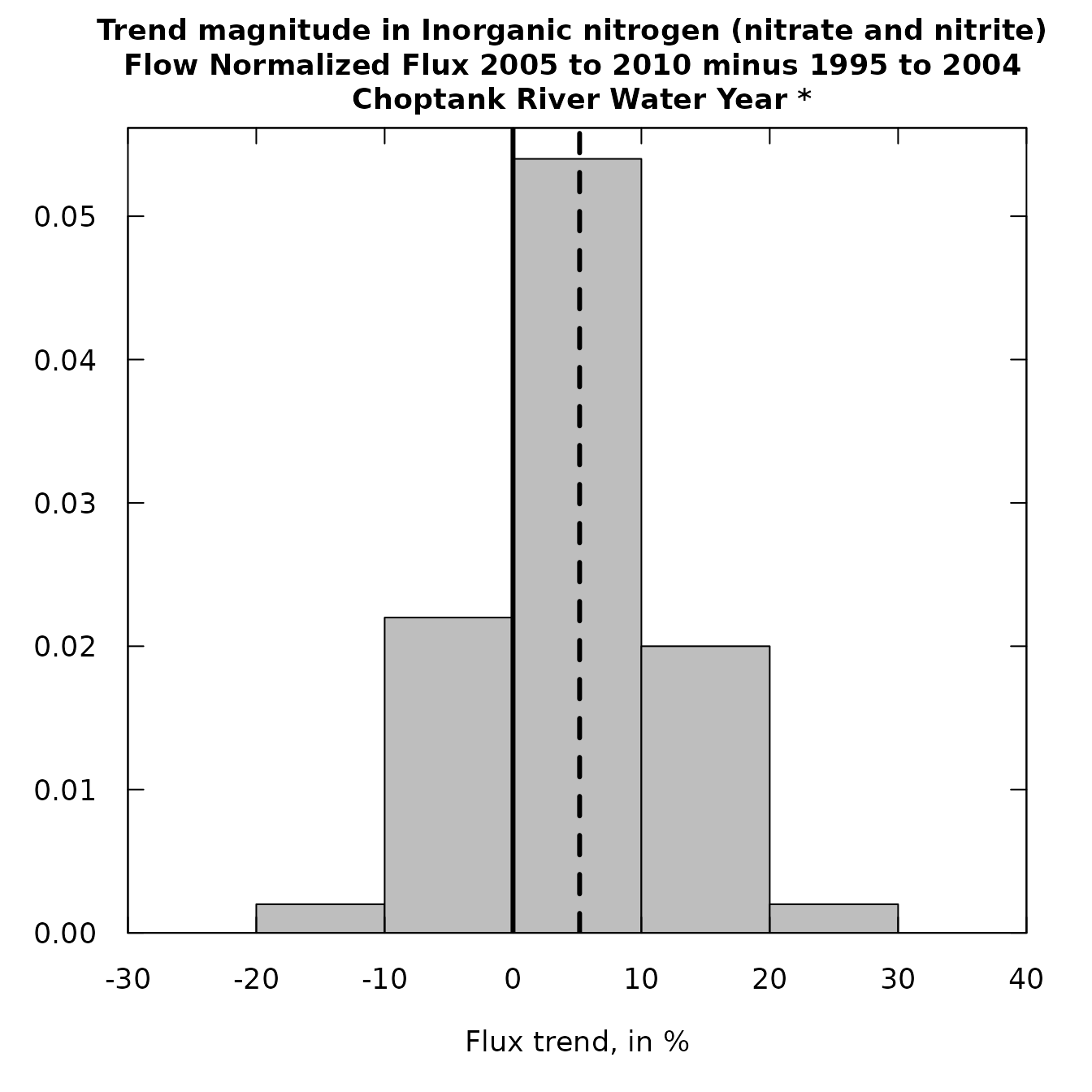
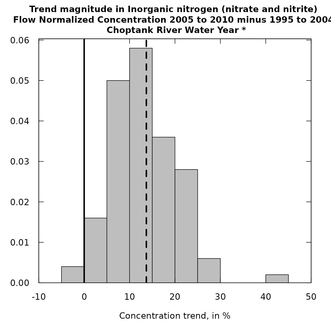
Here are the calls to plotHistogramTrend first for flux, and then for concentration. The xMin, xMax, and xStep arguments shown below were selected based on first viewing the results using the default values and then searching for a set of values for the three arguments that provided a good representation of the distribution.
plotHistogramTrend(eList, bootGroupsOut,
                   xMin = -30, xMax = 40, xStep = 10)
plotHistogramTrend(eList, bootGroupsOut,
                   flux=FALSE, xMin = -10,
                   xMax = 50, xStep = 5)
What the results clearly show us is that both flux and concentration indicate that it is somewhat more likely to have been an increase rather than a decrease between the two groups of years. Our best estimate is an increase is a little less than about + 10%. For both flux and concentration the trend is fairly likely to be in the range from -20% to about +30%.