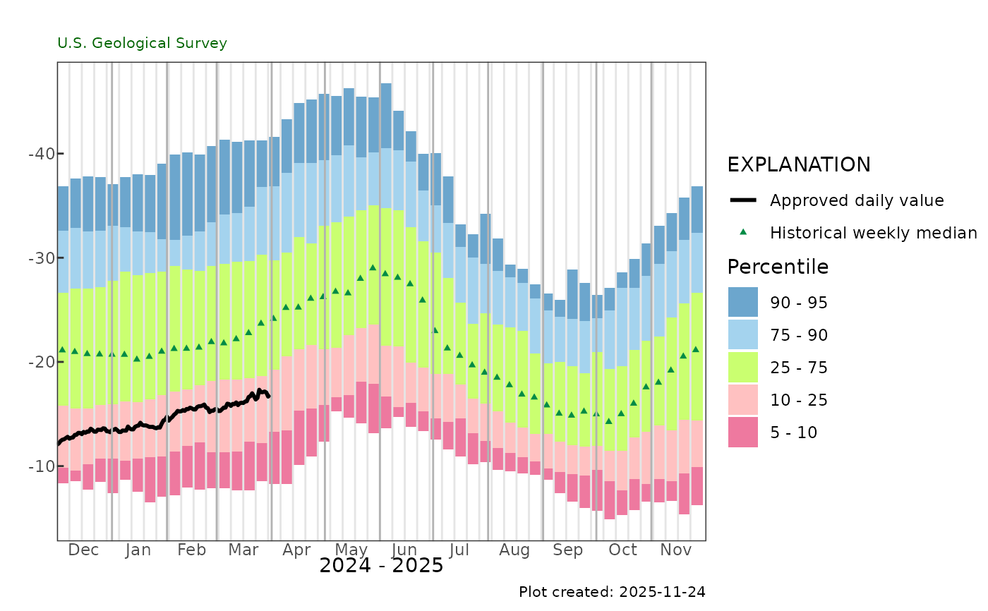
Plot weekly frequency analysis — weekly_frequency

Weekly statistics are calculated using the weekly_frequency_table function. Daily, discrete, or both types of data can be used.

Usage

weekly_frequency_plot(
  gw_level_dv,
  gwl_data,
  parameter_cd = NA,
  date_col = NA,
  value_col = NA,
  approved_col = NA,
  stat_cd = NA,
  plot_range = "Past year",
  plot_title = "",
  subtitle = "U.S. Geological Survey",
  y_axis_label = "",
  flip = FALSE,
  percentile_colors = NA
)

Arguments

gw_level_dv: data frame, daily groundwater level data. Often obtained from readNWISdv. Use NULL for no daily data.
gwl_data: data frame returned from readNWISgwl, or data frame with a date, value, and approval columns. Using the convention: lev_dt (representing date), lev_age_cd (representing approval code), and lev_va or sl_lev_va (representing value) will allow defaults to work. Use NULL for no discrete data.
parameter_cd: If data in gw_level_dv comes from NWIS, the parameter_cd can be used to define the value_col. If the data doesn't come directly from NWIS services, this can be set to NA,and this argument will be ignored.
date_col: the name of the date column. The default is NA, in which case, the code will try to get the column name automatically based on NWIS naming conventions. If both gw_level_dv and gwl_data data frames require custom column names, the first value of this input defines the date column for gw_level_dv, and the second defines gwl_data.
value_col: the name of the value column. The default is NA, in which case, the code will try to get the column name automatically based on NWIS naming conventions. If both gw_level_dv and gwl_data data frames require custom column names, the first value of this input defines the value column for gw_level_dv, and the second defines gwl_data.
approved_col: the name of the column to get provisional/approved status. The default is NA, in which case, the code will try to get the column name automatically based on NWIS naming conventions. If both gw_level_dv and gwl_data data frames require custom column names, the first value of this input defines the approval column for gw_level_dv, and the second defines gwl_data.
stat_cd: If data in gw_level_dv comes from NWIS, the stat_cd can be used to help define the value_col.
plot_range: the time frame to use for the plot. Either "Past year" to use the last year of data, or "Calendar year" to use the current calendar year, beginning in January.
plot_title: the title to use on the plot
subtitle: character. Sub-title for plot, default is "U.S. Geological Survey".
y_axis_label: the label used for the y-axis of the plot.
flip: logical. If TRUE, flips the y axis so that the smallest number is on top. Default is FALSE.
percentile_colors: Optional argument to provide a vector of 5 colors used to fill the percentile bars in order from lowest percentile bin to the highest percentile bin. Default behavior (NA) is to use legacy plot colors.

Value

a ggplot object with rectangles representing the historical weekly percentiles, and points representing the historical median and daily values

Examples


# site <- "263819081585801"
p_code_dv <- "62610"
statCd <- "00001"
# gw_level_dv <- dataRetrieval::readNWISdv(site, p_code_dv, statCd = statCd)
gw_level_dv <- L2701_example_data$Daily
weekly_frequency_plot(gw_level_dv,
                      gwl_data = NULL,
                      date_col = "Date",
                      value_col = "X_62610_00001",
                      approved_col = "X_62610_00001_cd")
#> Warning: Removed 5 rows containing missing values or values outside the scale range
#> (`geom_rect()`).
#> Warning: Removed 1 row containing missing values or values outside the scale range
#> (`geom_point()`).


gwl_data <- L2701_example_data$Discrete

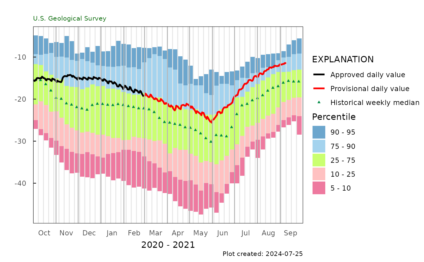weekly_frequency_plot(gw_level_dv,
                      gwl_data = gwl_data,
                      parameter_cd = "62610")
#> Warning: Removed 5 rows containing missing values or values outside the scale range
#> (`geom_rect()`).
#> Warning: Removed 1 row containing missing values or values outside the scale range
#> (`geom_point()`).


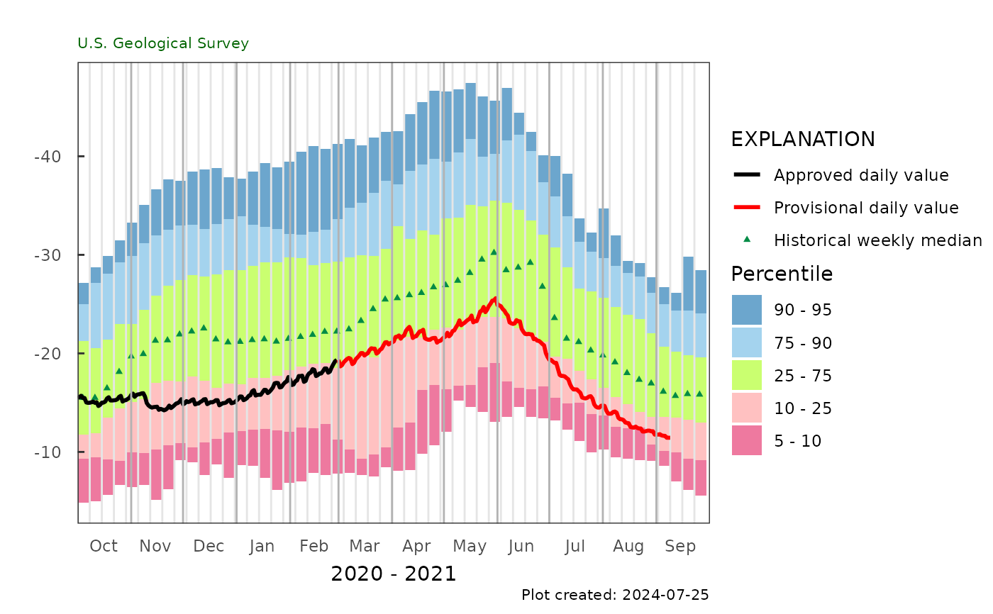weekly_frequency_plot(gw_level_dv,
                      gwl_data = gwl_data,
                      parameter_cd = "62610",
                      flip = TRUE)
#> Warning: Removed 5 rows containing missing values or values outside the scale range
#> (`geom_rect()`).
#> Warning: Removed 1 row containing missing values or values outside the scale range
#> (`geom_point()`).