Single Site Data Availability
Single_site_combo_data.RmdThis vignette shows how to use HASP and other R tools to
reproduce:
https://fl.water.usgs.gov/mapper/site_info.php?site=263819081585801&stationType=gw
This page merges information from USGS Groundwater Watch website and USGS Water Science Centers.
Site Information
library(HASP)

siteID <- "USGS-263819081585801"
site_metadata <- site_summary(siteID, markdown = TRUE)
USGS-263819081585801 L -2701
Lee County , Florida
Hydrologic Unit: 030902050603
Well depth: 206 feet
Land
surface altitude: 13 Level or other surveyed method.
Well completed
in : “Intermediate aquifer system” (S500INTRMD) national
aquifer.
data_info <- data_available(siteID)
kable(data_info)| Data Type | parameter_name | parameter_code | statistic_id | Begin Date | End Date |
|---|---|---|---|---|---|
| Daily | Elevation, GW, NGVD29 | 62610 | 00001 | 1978-10-01 | 2025-03-31 |
| Points | Elevation, GW, NGVD29 | 62610 | 00011 | 2007-10-01 | 2025-04-01 |
| Points | Elevation, GW, NAVD88 | 62611 | 00011 | 2022-12-05 | 2025-04-01 |
| Daily | Elevation, GW, NAVD88 | 62611 | 00001 | 2022-12-03 | 2025-03-31 |
| Field | Elevation, GW, NGVD29 | 62610 | 1982-10-12 | 2025-04-01 | |
| Field | Elevation, GW, NAVD88 | 62611 | 1982-10-12 | 2025-04-01 | |
| Field | Water level, depth LSD | 72019 | 1982-10-12 | 2025-04-01 | |
| Discrete Samples | Acid neutralizing capacity (ANC) as calcium carbonate, water, unfiltered, fixed endpoint (EP) (pH 4.5) titration, field | 00410 | 1978-09-06 | 1981-05-20 | |
| Discrete Samples | Acid neutralizing capacity (ANC) as calcium carbonate, water, unfiltered, fixed endpoint (EP) (pH 4.5) titration, laboratory | 95410, 00417, 90410 | 1981-05-20 | 1984-04-12 | |
| Discrete Samples | Agency analyzing sample | 00028 | 1978-09-06 | 2006-04-11 | |
| Discrete Samples | Bicarbonate as bicarbonate, water, unfiltered, fixed endpoint (EP) (pH 4.5) titration, field | 00440 | 1978-09-06 | 1979-05-09 | |
| Discrete Samples | Bicarbonate as bicarbonate, water, unfiltered, inflection-point titration, laboratory | 00449, 90440 | 1982-06-03 | 1982-06-03 | |
| Discrete Samples | Calcium, water, filtered | 00915, 91051 | 1978-09-06 | 1984-04-12 | |
| Discrete Samples | Carbon dioxide, water, unfiltered | 00405 | 1978-09-06 | 1981-05-20 | |
| Discrete Samples | Carbonate as carbonate, water, unfiltered, fixed endpoint (EP) (pH 8.3) titration, field | 00445 | 1978-09-06 | 1979-05-09 | |
| Discrete Samples | Carbonate as carbonate, water, unfiltered, inflection-point titration, laboratory | 90445, 00446 | 1982-06-03 | 1982-06-03 | |
| Discrete Samples | Chloride, water, filtered | 00940, 91001 | 1978-09-06 | 2011-04-20 | |
| Discrete Samples | Chloride, water, unfiltered | 99220 | 2011-10-17 | 2022-05-18 | |
| Discrete Samples | Color, water, filtered | 00080 | 1978-09-06 | 1984-04-12 | |
| Discrete Samples | Depth of well, below land surface datum (LSD) | 72008 | 2012-05-02 | 2012-05-02 | |
| Discrete Samples | Depth to bottom, at sampling location | 81903 | 1998-11-18 | 2000-07-12 | |
| Discrete Samples | Dissolved oxygen (DO), water, unfiltered | 00300 | 1998-11-18 | 1998-11-18 | |
| Discrete Samples | Dissolved solids, water, filtered | 70303 | 1978-09-06 | 1984-04-12 | |
| Discrete Samples | Dissolved solids, water, filtered, dried at 180 degrees Celsius | 70300 | 1978-09-06 | 1984-04-12 | |
| Discrete Samples | Dissolved solids, water, filtered, sum of constituents | 70301 | 1978-09-06 | 1984-04-12 | |
| Discrete Samples | Elevation of water surface, groundwater, above NGVD 1929 | 62610 | 2015-10-22 | 2018-05-04 | |
| Discrete Samples | Elevation, above NGVD 1929 | 30211, 72020, 99020 | 1982-10-12 | 2010-03-22 | |
| Discrete Samples | Fluoride, water, filtered | 91002, 00950 | 1978-09-06 | 1984-04-12 | |
| Discrete Samples | Hardness as calcium carbonate, water | 00900 | 1978-09-06 | 1984-04-12 | |
| Discrete Samples | Hydrogen ion, water, unfiltered, calculated | 00191 | 1978-09-06 | 2000-07-12 | |
| Discrete Samples | Iron, water, filtered | 52777, 01046 | 1978-09-06 | 1984-04-12 | |
| Discrete Samples | Magnesium, water, filtered | 91052, 00925 | 1978-09-06 | 1984-04-12 | |
| Discrete Samples | Noncarbonate hardness as calcium carbonate, water | 95902 | 1981-05-20 | 1981-05-20 | |
| Discrete Samples | Noncarbonate hardness as calcium carbonate, water, unfiltered, field | 00902 | 1978-09-06 | 1981-05-20 | |
| Discrete Samples | pH, water, unfiltered, field | 00400 | 1978-09-06 | 2000-07-12 | |
| Discrete Samples | pH, water, unfiltered, laboratory | 00403 | 1981-05-20 | 1984-04-12 | |
| Discrete Samples | Potassium-40, water, filtered | 82068 | 1981-05-20 | 1981-05-20 | |
| Discrete Samples | Potassium, water, filtered | 00935, 91054 | 1978-09-06 | 1984-04-12 | |
| Discrete Samples | Salinity, water, unfiltered, normalized to 25 degrees Celsius | 00096, 90860 | 1998-11-18 | 2000-05-16 | |
| Discrete Samples | Sampling condition | 72006 | 2019-04-17 | 2022-05-18 | |
| Discrete Samples | Sampling depth | 00003, 00098 | 2013-04-22 | 2022-05-18 | |
| Discrete Samples | Silica as silicon dioxide, water, filtered | 68809, 00955 | 1978-09-06 | 1984-04-12 | |
| Discrete Samples | Sodium adsorption ratio (SAR), water | 00931 | 1978-09-06 | 1984-04-12 | |
| Discrete Samples | Sodium fraction of cations, water | 00932 | 1978-09-06 | 1984-04-12 | |
| Discrete Samples | Sodium, water, filtered | 91053, 00930 | 1978-09-06 | 1984-04-12 | |
| Discrete Samples | Source of sample | 72005 | 2022-05-18 | 2022-05-18 | |
| Discrete Samples | Specific conductance, water, unfiltered, normalized to 25 degrees Celsius | 00094, 00095 | 1979-05-09 | 2022-05-18 | |
| Discrete Samples | Specific conductance, water, unfiltered, normalized to 25 degrees Celsius, laboratory | 90095 | 1981-05-20 | 2022-05-18 | |
| Discrete Samples | Strontium, water, filtered | 01080 | 1978-09-06 | 1984-04-12 | |
| Discrete Samples | Sulfate, water, filtered | 91005, 00945 | 1978-09-06 | 1984-04-12 | |
| Discrete Samples | Temperature, water | 00010, 00011 | 1978-09-06 | 2022-05-18 |
Get data using dataRetrieval
Using dataRetrieval code to get the data for this
site:
library(dataRetrieval)
siteID <- "USGS-263819081585801"
parameterCd <- "62610"
statCd <- "00001"
# Daily data:
gw_level_dv <- read_waterdata_daily(monitoring_location_id = siteID,
                                    parameter_code = parameterCd,
                                    statistic_id = statCd,
                                    skipGeometry = TRUE)

# Field measured:
gwl_data <- dataRetrieval::read_waterdata_field_measurements(monitoring_location_id = siteID,
                                                             skipGeometry = TRUE)

# Water quality data:
cl_sc <- c("Chloride", "Specific conductance")
qw_data <- readWQPqw(siteNumbers = siteID,
                     parameterCd = cl_sc)

plot_title <- "L -2701\n263819081585801"
y_label <- dataRetrieval::read_waterdata_parameter_codes(parameter_code = parameterCd)$parameter_name
Groundwater Data
Monthly Frequency
monthly_frequency_plot(gw_level_dv,
                       gwl_data = gwl_data,
                       parameter_cd = parameterCd,
                       y_axis_label = y_label,
                       plot_title = plot_title,
                       plot_range = "Past year")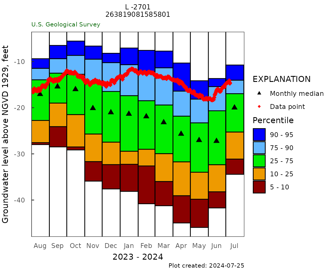
monthly_freq_table <- monthly_frequency_table(gw_level_dv,
                                              gwl_data,
                                              parameter_cd = parameterCd)
kable(monthly_freq_table, digits = 1)| month | p05 | p10 | p25 | p50 | p75 | p90 | p95 | nYears | minMed | maxMed |
|---|---|---|---|---|---|---|---|---|---|---|
| 1 | -37.6 | -32.2 | -29.4 | -20.3 | -17.2 | -11.0 | -7.2 | 47 | -41.8 | -5.7 |
| 2 | -40.4 | -32.6 | -28.9 | -21.4 | -17.7 | -12.3 | -7.6 | 47 | -42.9 | -7.2 |
| 3 | -41.0 | -35.6 | -29.9 | -22.9 | -18.8 | -12.1 | -7.8 | 47 | -45.2 | -6.9 |
| 4 | -44.5 | -39.0 | -31.4 | -25.1 | -21.6 | -15.1 | -10.5 | 47 | -48.4 | -9.4 |
| 5 | -45.7 | -39.8 | -33.8 | -27.0 | -23.2 | -17.6 | -14.2 | 46 | -49.4 | -10.0 |
| 6 | -41.6 | -37.8 | -32.3 | -26.7 | -20.2 | -15.6 | -13.7 | 45 | -42.8 | -11.0 |
| 7 | -34.3 | -31.1 | -24.7 | -19.9 | -16.7 | -13.6 | -10.8 | 46 | -37.5 | -6.8 |
| 8 | -28.0 | -27.6 | -22.6 | -17.0 | -13.8 | -10.9 | -9.4 | 46 | -32.4 | -4.8 |
| 9 | -28.3 | -24.1 | -19.0 | -15.4 | -12.0 | -9.4 | -6.6 | 45 | -32.7 | -3.2 |
| 10 | -29.1 | -28.5 | -21.3 | -16.0 | -12.6 | -8.3 | -5.6 | 47 | -36.2 | -4.8 |
| 11 | -35.7 | -31.5 | -25.6 | -20.1 | -14.5 | -9.6 | -6.7 | 47 | -41.4 | -4.5 |
| 12 | -37.2 | -32.1 | -27.4 | -20.9 | -16.0 | -10.4 | -8.3 | 47 | -42.5 | -4.9 |
Daily 2 year plot
daily_gwl_plot(gw_level_dv,
               gwl_data,
               parameter_cd = parameterCd,
               plot_title = plot_title,
               month_breaks = TRUE,
               historical_stat = "median",
               y_axis_label = y_label)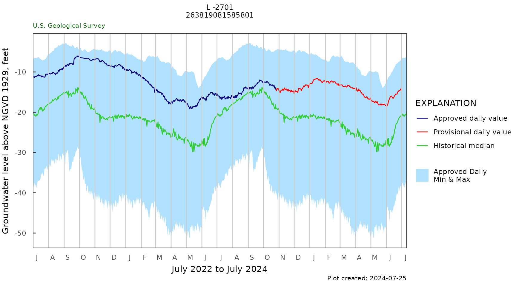
daily_summary_table <- daily_gwl_summary(gw_level_dv,
                                         gwl_data,
                                         parameter_cd = parameterCd) |>
  select("Begin Date" = begin_date,
         "End Date" = end_date,
         "Days" = days,
         "% Complete" = percent_complete,
         "Lowest Level" = lowest_level,
         "25th" = p25,
         "50th" = p50,
         "75th" = p75,
         "Highest Level" = highest_level)
kable(t(daily_summary_table))| Begin Date | 1978-10-01 |
| End Date | 2025-04-01 |
| Days | 16762 |
| % Complete | 99 |
| Lowest Level | -51.3 |
| 25th | -27.67 |
| 50th | -21.1 |
| 75th | -15.83 |
| Highest Level | -2.81 |
Field Groundwater Level Data
gwl_plot_field(gwl_data,
               parameter_cd = parameterCd,
               plot_title = plot_title,
               flip = FALSE)
siteField <- gwl_data |>
  site_data_summary(site_col = "monitoring_location_id")

kable(siteField, digits = 1)| site | min_site | max_site | mean_site | p10 | p25 | p50 | p75 | p90 | count |
|---|---|---|---|---|---|---|---|---|---|
| USGS-263819081585801 | -52.4 | 64.3 | -4.6 | -34.8 | -29 | -20.1 | 32.5 | 43.2 | 1461 |
Period of Record - All Data Types
y_label <- dataRetrieval::read_waterdata_parameter_codes(parameter_code = parameterCd)$parameter_name

gwl_plot_all(gw_level_dv,
             gwl_data,
             y_label = y_label,
             plot_title = plot_title,
             parameter_cd = parameterCd,
             flip = FALSE)
siteDaily <- gw_level_dv |>
  site_data_summary() |>
  select(Minimum = min_site,
         `1st` = p25,
         Median = p50,
         Mean = mean_site,
         `3rd` = p75,
         Maximum = max_site)

kable(siteDaily, digits = 1)| Minimum | 1st | Median | Mean | 3rd | Maximum |
|---|---|---|---|---|---|
| -51.1 | -27.5 | -21 | -21.9 | -15.8 | -2.8 |
Salinity Data and Analysis
Chloride
qw_plot(qw_data, plot_title = plot_title)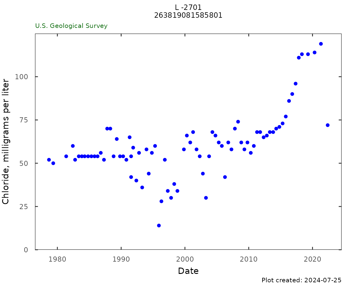
cl_trend <- trend_test(gw_level_dv = NULL,
                      gwl_data = dplyr::filter(qw_data,
                   CharacteristicName == "Chloride"),
                     approved_col = c(NA, "ResultStatusIdentifier"),
                     date_col = c(NA, "ActivityStartDateTime"),
                     value_col = c(NA, "ResultMeasureValue"))
kable(cl_trend, digits = 3)| test | tau | pValue | slope | intercept | trend |
|---|---|---|---|---|---|
| 10-year trend | 0.838 | 0 | 6.521 | -13071.910 | Up |
| Period of record | 0.483 | 0 | 0.647 | -1237.109 | Up |
chl_table <- qw_summary(qw_data,
                        CharacteristicName = "Chloride",
                        norm_range = c(225,999))
kable(chl_table)| Analysis | Result |
|---|---|
| Date of first sample | 1978-09-06 |
| First sample result (mg/l) | 52 |
| Date of last sample | 2022-05-18 |
| Last sample result (mg/l) | 72 |
| Date of first sample within 225 to 999 mg/l | |
| Date of first sample with 1000 mg/l or greater | |
| Minimum (mg/l) | 14 |
| Maximum (mg/l) | 119 |
| Mean (mg/l) | 60.9 |
| First quartile (mg/l) | 54 |
| Median (mg/l) | 58 |
| Third quartile (mg/l) | 68 |
| Number of samples | 81 |
Specific Conductance
qw_plot(qw_data, "Specific Conductance",
        CharacteristicName = "Specific conductance")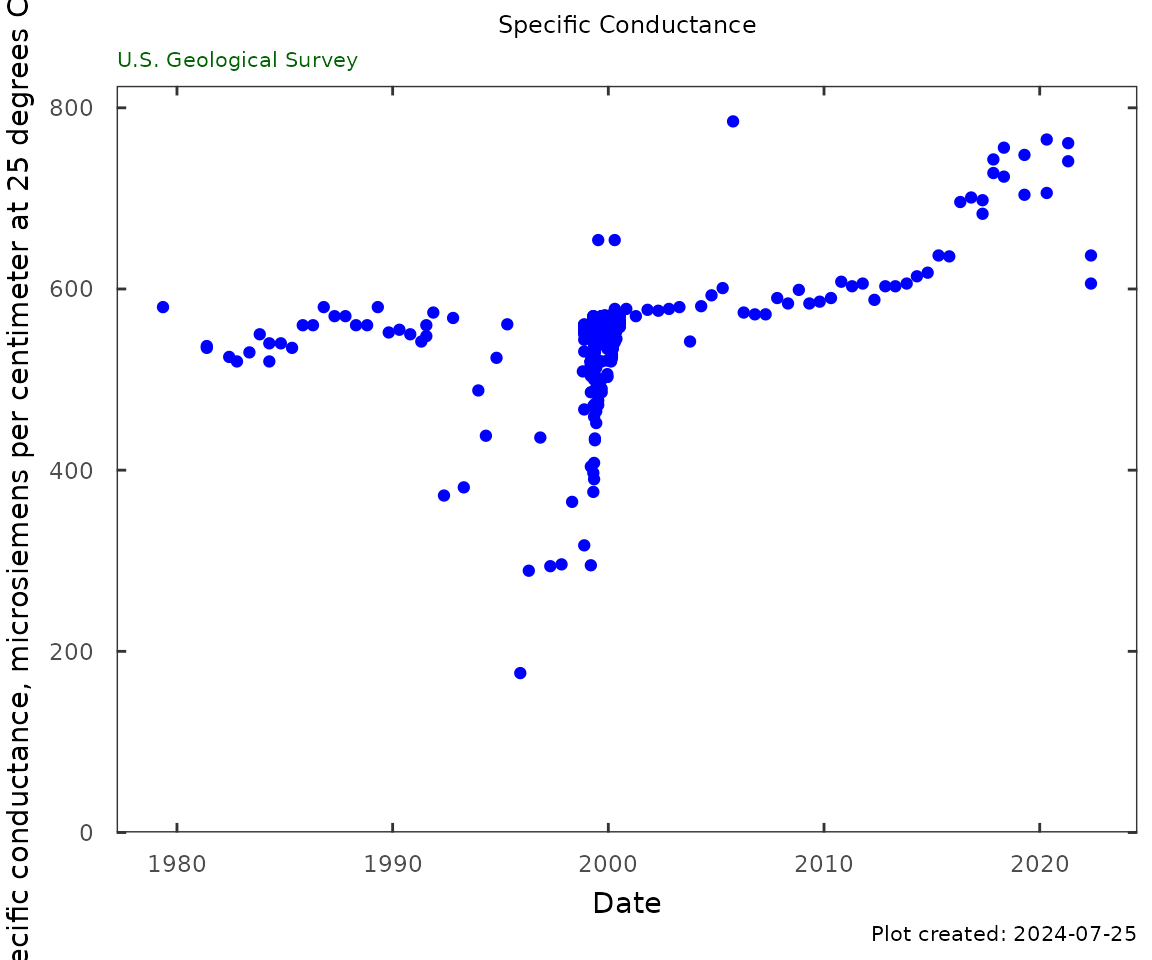
sc_table <- qw_summary(qw_data,
                       CharacteristicName = "Specific conductance",
                       norm_range = NA)
kable(sc_table)| Analysis | Result |
|---|---|
| Date of first sample | 1979-05-09 |
| First sample result (uS/cm @25C) | 580 |
| Date of last sample | 2022-05-18 |
| Last sample result (uS/cm @25C) | 606 |
| Minimum (uS/cm @25C) | 176 |
| Maximum (uS/cm @25C) | 785 |
| Mean (uS/cm @25C) | 553 |
| First quartile (uS/cm @25C) | 544 |
| Median (uS/cm @25C) | 560 |
| Third quartile (uS/cm @25C) | 569 |
| Number of samples | 394 |
Specific Conductance vs Chloride
Sc_Cl_plot(qw_data, plot_title = plot_title)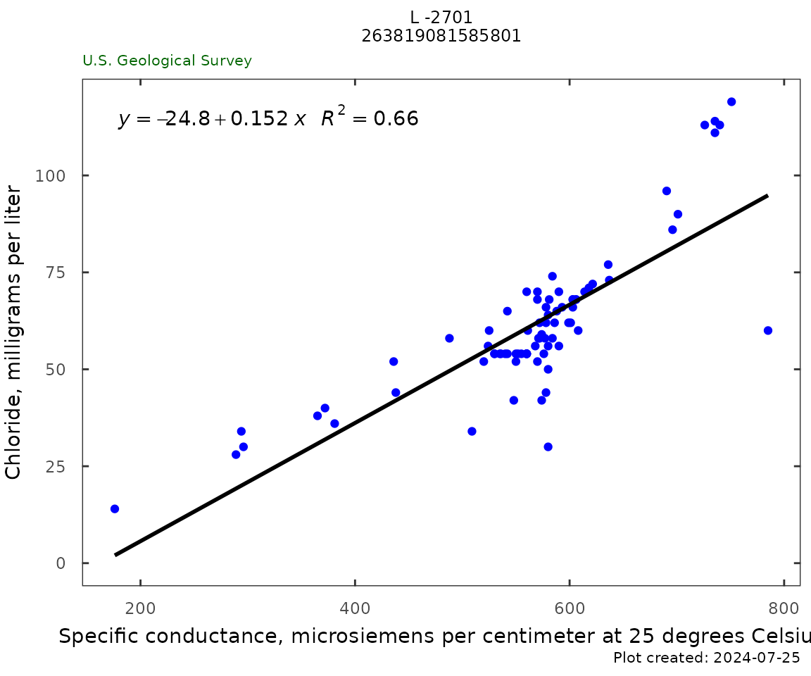
sc_cl <- Sc_Cl_table(qw_data)

# only show 10 row:
kable(head(sc_cl, 10),
      col.names = c("Date",
                    "Chloride [mg/L]",
"Specific conductance [µS/L]"))| Date | Chloride [mg/L] | Specific conductance [µS/L] |
|---|---|---|
| 1978-09-06 20:30:00 | 52 | |
| 1979-05-09 19:00:00 | 50 | 580 |
| 1981-05-20 18:15:00 | 54 | 536 |
| 1982-06-03 13:30:00 | 60 | 525 |
| 1982-10-12 13:15:00 | 52 | 520 |
| 1983-05-11 15:50:00 | 54 | 530 |
| 1983-11-02 16:30:00 | 54 | 550 |
| 1984-04-12 16:30:00 | 54 | 530 |
| 1984-10-24 14:05:00 | 54 | 540 |
| 1985-05-03 19:45:00 | 54 | 535 |