USGS Water Quality Data
Introduction to dataRetrieval

Laura DeCicco

Introduction

In this ~90 minute introduction, the goal is:

• Introduce the modern dataRetrieval workflows.

• The intended audience is someone:

  • New to dataRetrieval

  • Has some R experience

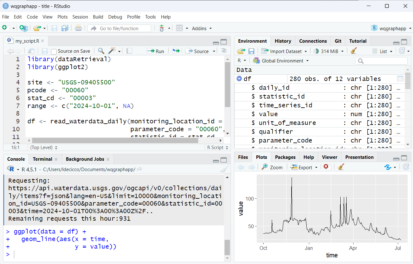
RStudio Orientation

By default will look like:

RStudio Appearances

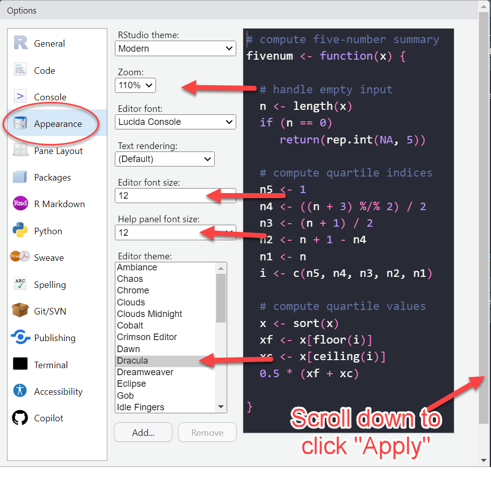
Go to Tools -> Global Options -> Appearances to change style.

RStudio Orientation

1. Create scripts.

2. See code run.

3. See what variables are loaded

• Click on a data frame to View

4. Plots and more

dataRetrieval: R-package for US water data

USGS Water Data APIs *

• Surface water levels

• Groundwater levels

• Site metadata

• Peak flows

• Rating curves

• Discrete water-quality data

Water Quality Portal (WQP) Data

• Discrete water-quality data

• USGS and non-USGS data

Installation

dataRetrieval is available on the Comprehensive R Archive Network (CRAN) repository. To install dataRetrieval on your computer, open RStudio and run this line of code in the Console:

install.packages("dataRetrieval")

Then each time you open R, you’ll need to load the library:

library(dataRetrieval)

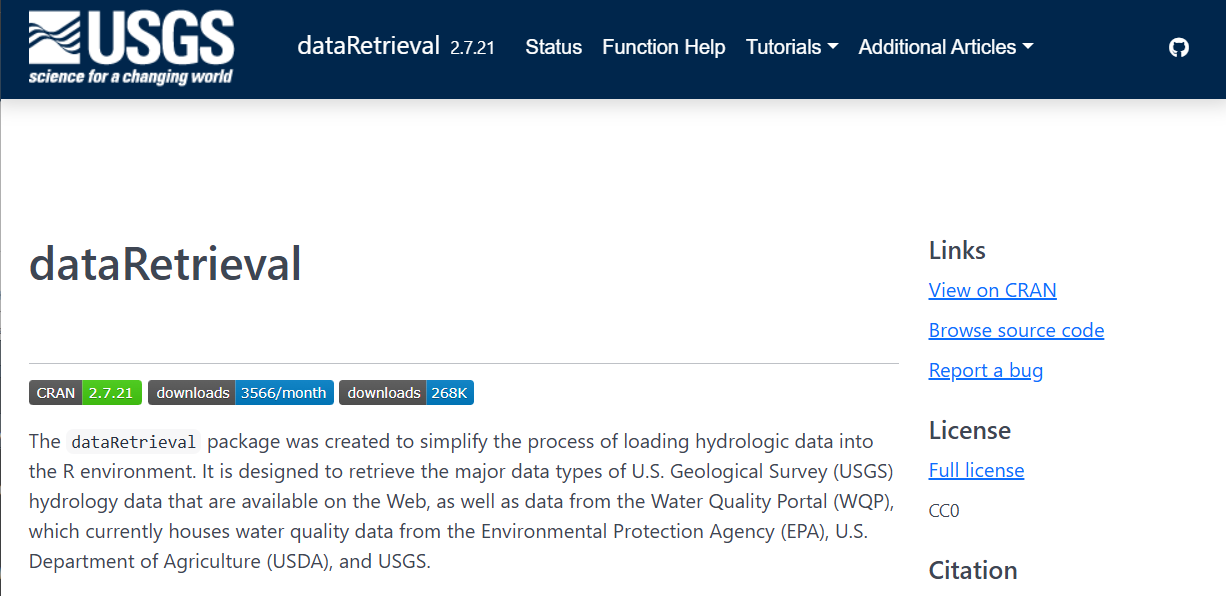
dataRetrieval: External Documentation

dataRetrieval: External Documentation

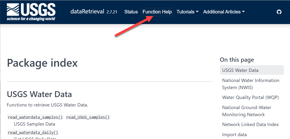
dataRetrieval: External Documentation

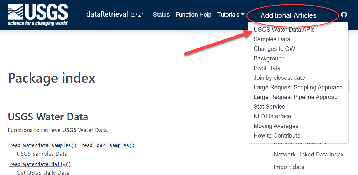
Documentation within R: function help pages

Within R, you can call help files for any dataRetrieval function:

?readWQPdata

Click here to open a new window:

Scroll down to the “Examples” to see how each function can be run.

Examples

# Legacy:
nameToUse <- "pH"
pHData <- readWQPdata(siteid = "USGS-04024315", 
                      characteristicName = nameToUse)
ncol(pHData)
attr(pHData, "siteInfo")
attr(pHData, "queryTime")
attr(pHData, "url")

Exercise 1: Orientation

• Challenge
• Solution:

1. Open RStudio

2. Install dataRetrieval, dplyr, ggplot2, and data.table (if they are not already installed).

3. Load dataRetrieval

4. Open the help file for the function read_waterdata_daily

5. Navigate to https://doi-usgs.github.io/dataRetrieval/ and find the list of function help files and explore some articles in “Additional Articles”

install.packages(c("dataRetrieval", "dplyr", "ggplot2", "data.table"))
library(dataRetrieval)
?read_waterdata_daily

dataRetrieval Updates

Are you a seasoned dataRetrieval user?

Here are resources for recent major changes:

• Changes to dataRetrieval

• Water Data API Introduction

• Samples Data Introduction

What’s New?

There’s been a lot of changes to dataRetrieval over the past year. If you’d like to see an overview of those changes, visit: Changes to dataRetrieval

Biggest changes:

• NWIS servers will be shut down, so all readNWIS functions will eventually stop working

• read_waterdata functions are modern and should be used when possible

• The “USGS Water Data APIs” are the new home for USGS data

USGS Water Data API Token

• The Water Data APIs limit how many queries a single IP address can make per hour

• You can run new dataRetrieval functions without a token

• You might run into errors quickly. If you (or your IP!) have exceeded the quota, you will see:

! HTTP 429 Too Many Requests.
  • You have exceeded your rate limit. Make sure you provided your API key from https://api.waterdata.usgs.gov/signup/, then either try again later or contact us at https://waterdata.usgs.gov/questions-comments/?referrerUrl=https://api.waterdata.usgs.gov for assistance.

USGS Water Data API Token

1. Request a USGS Water Data API Token: https://api.waterdata.usgs.gov/signup/

2. Save it in a safe place (KeePass or other password management tool)

3. Add it to your .Renviorn file as API_USGS_PAT.

4. Restart R

5. Check that it worked by running (you should see your token printed in the Console):

Sys.getenv("API_USGS_PAT")

See next slide for a demonstration.

USGS Water Data API Token: Example

My favorite method to do add your token to .Renviron is to use the usethis package. Let’s pretend the token sent you was “abc123”:

1. Run in R:

usethis::edit_r_environ()

2. Add this line to the file that opens up:

API_USGS_PAT = "abc123"

3. Save that file using the save button

4. Restart R/RStudio.

5. Run after restarting R:

Sys.getenv("API_USGS_PAT")

USGS Water Data API Token: Example

After save and restart, check that it worked by running:

Sys.getenv("API_USGS_PAT")

USGS Basic Retrievals

The USGS uses various codes for basic retrievals. These codes can have leading zeros, therefore they need to be a character surrounded in quotes (“00060”).

• Site ID (often 8 or 15-digits)
• Parameter Code (5 digits)
  • Full list: read_waterdata_parameter_codes()
• Statistic Code (for daily values)
  • Full list: read_metadata("statistic-codes")

USGS Basic Retrievals Parameter and Statistic Codes

Here are some examples of a few common codes:

Parameter Code Short Name 00060 Discharge 00065 Gage Height 00010 Temperature 00400 pH

Statistic Code Short Name 00001 Maximum 00002 Minimum 00003 Mean 00008 Median

Let’s Go!

We’re going walk through 3 retrievals:

• Workflow 1: Daily Data

  • Uses the new USGS Water Data API

  • Modern data access point going forward

• Workflow 2: Discrete Data

  • Uses new USGS Samples Data

  • Modern data access point going forward

• Workflow 3: Join Daily and Discrete

• Workflow 4: Continuous Data

  • Uses the NWIS web services

  • Will be deprecated, this fall we’ll have read_waterdata_continuous

• Workflow 5: Join Continuous and Discrete

Workflow 1: Daily data for known site

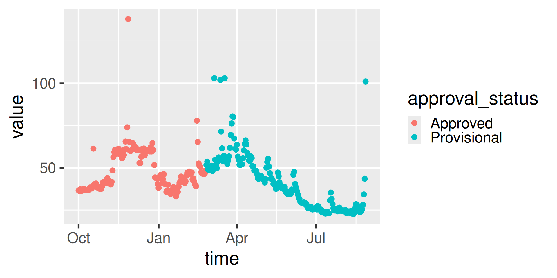
Let’s pull daily mean discharge data for site “USGS-0940550”, getting all the data from October 10, 2024 onward.

library(dataRetrieval)
site <- "USGS-09405500"
pcode <- "00060" # Discharge
stat_cd <- "00003" # Mean
range <- c("2024-10-01", NA)

df <- read_waterdata_daily(monitoring_location_id = site,
                           parameter_code = pcode,
                           statistic_id = stat_cd,
                           time = range)

Requesting:
https://api.waterdata.usgs.gov/ogcapi/v0/collections/daily/items?f=json&lang=en-US&limit=10000&monitoring_location_id=USGS-09405500&parameter_code=00060&statistic_id=00003&time=2024-10-01%2F..

Remaining requests this hour:137 

Workflow 1: Look at Daily Data

In RStudio, click on the data frame in the upper right Environment tab to open a Viewer.

Workflow 1: Plot Daily Data

Let’s use ggplot2 to visualize the data.

library(ggplot2)

ggplot(data = df) +
  geom_point(aes(x = time, 
                 y = value,
                 color = approval_status)) 

Water Data API Notes: Argument input

Use your “tab” key!

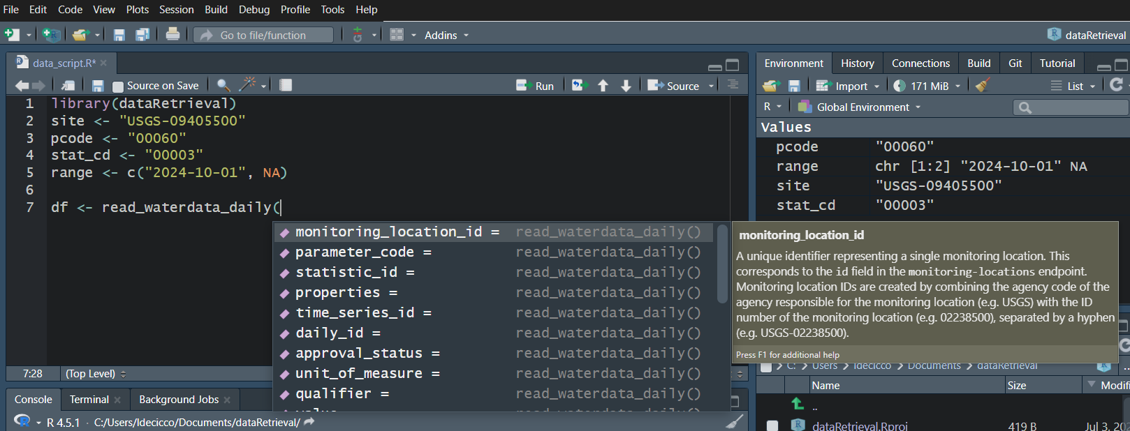
Water Data API Notes: Arguments

• When you look at the help file for the new functions, you’ll notice there are lots of possible inputs (arguments).

• You DO NOT need to (and should not!) specify all of these parameters.

• However, also consider what happens if you leave too many things blank. What do you suppose will be returned here?

discharge <- read_waterdata_daily(parameter_code = "00060",
                                  statistic_id = "00003")

Since no list of sites or bounding box was defined, ALL the daily data in ALL the country with parameter code “00060” and statistic code “00003” will be returned.

Water Data API Notes: time input

The “time” argument has a few options:

• A single date (or date-time): “2024-10-01” or “2024-10-01T23:20:50Z”

• A bounded interval: c(“2024-10-01”, “2025-07-02”)

• Half-bounded intervals: c(“2024-10-01”, NA)

• Duration objects: “P1M” for data from the past month or “PT36H” for the last 36 hours

Here are a bunch of valid inputs:

# Ask for exact times:
time = "2025-01-01"
time = as.Date("2025-01-01")
time = "2025-01-01T23:20:50Z"
time = as.POSIXct("2025-01-01T23:20:50Z", 
                  format = "%Y-%m-%dT%H:%M:%S", 
                  tz = "UTC")
# Ask for specific range
time = c("2024-01-01", "2025-01-01") # or Dates or POSIXs
# Asking beginning of record to specific end:
time = c(NA, "2024-01-01") # or Date or POSIX
# Asking specific beginning to end of record:
time = c("2024-01-01", NA) # or Date or POSIX
# Ask for period
time = "P1M" # past month
time = "P7D" # past 7 days
time = "PT12H" # past hours

Workflow 2: Discrete data for known site

Use your “tab” key!

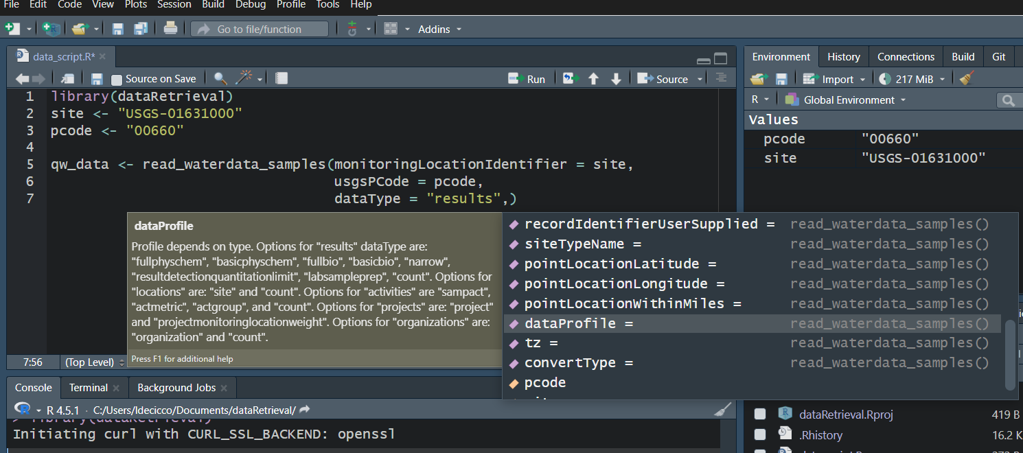
Workflow 2: Discrete data for known site

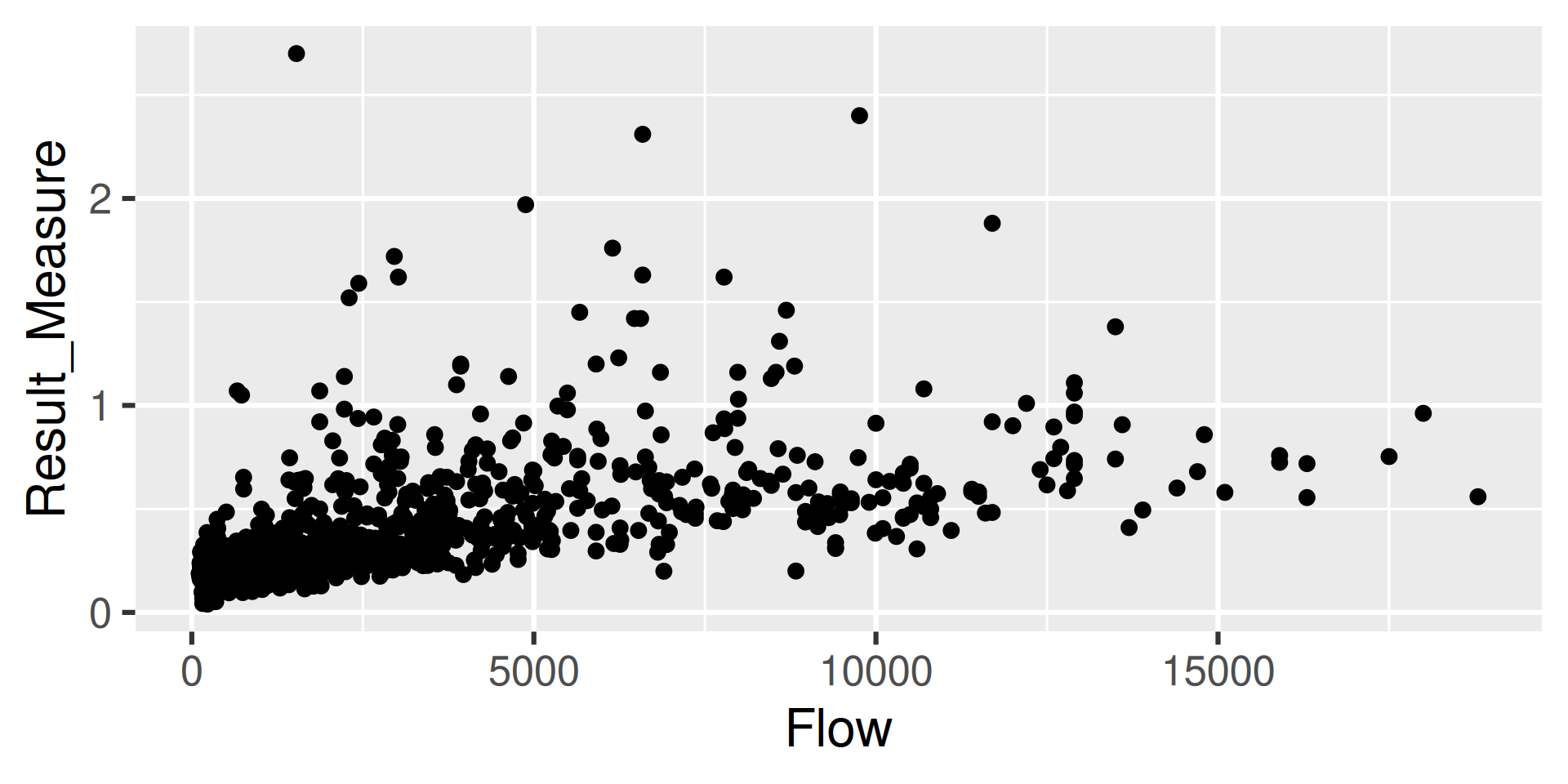
Let’s get orthophosphate (“00660”) data from the Shenandoah River at Front Royal, VA (“USGS-01631000”).

site <- "USGS-01631000"
pcode <- "00660"

qw_data <- read_waterdata_samples(monitoringLocationIdentifier = site,
                                  usgsPCode = pcode, 
                                  dataType = "results", 
                                  dataProfile = "basicphyschem")

GET: https://api.waterdata.usgs.gov/samples-data/results/basicphyschem?mimeType=text%2Fcsv&monitoringLocationIdentifier=USGS-01631000&usgsPCode=00660

ncol(qw_data)

[1] 100

That’s a LOT of columns that come back. We won’t look at them here, but you can use View in RStudio to explore on your own.

USGS Samples Data Notes: Data Types and Profiles

• There are 2 arguments that dictate what kind of data is returned
  • “dataType” defines what kind of data comes back
  • “dataProfile” defines what columns from that type come back

Data Types and Profiles

Workflow 2: Discrete data censoring

Let’s pull a few columns out and look at those:

library(dplyr)

qw_data_slim <- qw_data |> 
  select(Date = Activity_StartDate,
         Result_Measure,
         DL_cond = Result_ResultDetectionCondition,
         DL_val = DetectionLimit_MeasureA,
         DL_type = DetectionLimit_TypeA) |> 
  mutate(Result = if_else(!is.na(DL_cond), DL_val, Result_Measure),
         Detected = if_else(!is.na(DL_cond), "Not Detected", "Detected")) |> 
  arrange(Detected)

• What is |>? It’s a pipe! It says take ‘this thing’ and put it in ‘that thing’. You’ll also see %>% in code, it is also a pipe - they are basically the same.

Workflow 2: Discrete data censoring information

Workflow 3: Join Discrete and Daily

• One common workflow is to join discrete data with daily data.

• In this example, we will look at a site that measures both water quality parameters and has daily mean discharge.

• We will use the dplyr::left_join to join the 2 data frames by a date.

Step 1: Get the data

site <- "USGS-04183500"
p_code_dv <- "00060"
stat_cd <- "00003"
p_code_qw <- "00665"
start_date <- "2015-07-03"
end_date <- "2025-07-03"

qw_data <- read_waterdata_samples(monitoringLocationIdentifier = site,
                             usgsPCode = p_code_qw, 
                             activityStartDateLower = start_date,
                             activityStartDateUpper = end_date,
                             dataProfile = "basicphyschem")

dv_data <- read_waterdata_daily(monitoring_location_id = site, 
                      parameter_code = p_code_dv,
                      statistic_id = stat_cd,
                      time = c(start_date, end_date))

Step 2: Join

library(dplyr)

little_dv <- dv_data |>
  select(time, Flow = value, monitoring_location_id)

qw_data_joined <- qw_data |> 
  left_join(little_dv, 
            by = c("Activity_StartDate" = "time"))

• “Activity_StartDate” (on the left side data frame) and “time” (on the right side data frame) need to be the same type (in this case, both are Date objects).

Step 2: Join (cont.)

• You could join on multiple columns:

qw_data <- qw_data |> 
  left_join(little_dv, 
            by = c("Activity_StartDate" = "time",
                   "Location_Identifier" = "monitoring_location_id"))

See dplyr documentation for lots of joining options, but I find left_join my “go-to” for straightforward joins.

Step 3: Inspect

Let’s take a quick peak:

ggplot(data = qw_data_joined) +
  geom_point(aes(x = Flow, 
                 y = Result_Measure))

Exercise 2: Joins

• Challenge
• Solution:

dplyr comes with some data sets. To look at them run:

library(dplyr)
band_members <- band_members
band_instruments <- band_instruments

1. Run that code and view the 2 data frames to see what they look like.

2. Join the instruments to the “band_members” by name.

3. Join the members to the “band_instruments” by name.

band_members |> 
  left_join(band_instruments, by = "name")

# A tibble: 3 × 3
  name  band    plays 
  <chr> <chr>   <chr> 
1 Mick  Stones  <NA>  
2 John  Beatles guitar
3 Paul  Beatles bass  

band_instruments |> 
  left_join(band_members, by = "name")

# A tibble: 3 × 3
  name  plays  band   
  <chr> <chr>  <chr>  
1 John  guitar Beatles
2 Paul  bass   Beatles
3 Keith guitar <NA>   

Workflow 4: Continuous data for known site

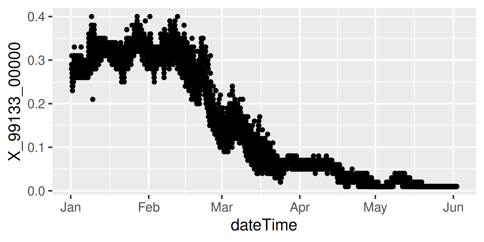
• Continuous data is the high-frequency sensor data.

• The function to get that data today is readNWISuv

• As NWIS gets deprecated, we expect to have read_waterdata_continuous soon

• We’ll look at Suisun Bay a Van Sickle Island NR Pittsburg CA (“USGS-11455508”), with parameter code “99133” which is Nitrate plus Nitrite.

Workflow 4: Continuous data for known site

site_id <- "11455508"
p_code_rt <- "99133"
start_date <- "2024-01-01"
end_date <- "2024-06-01"

continuous_data <- readNWISuv(site_id,
                              p_code_rt,
                              start_date,
                              end_date)
                 
names(continuous_data)

[1] "agency_cd"        "site_no"          "dateTime"         "X_99133_00000"   
[5] "X_99133_00000_cd" "tz_cd"           

[1] "agency_cd"       
[2] "site_no"         
[3] "dateTime"        
[4] "X_99133_00000"   
[5] "X_99133_00000_cd"
[6] "tz_cd" 

GET: https://nwis.waterservices.usgs.gov/nwis/iv/?site=11455508&format=waterml%2C1.1&ParameterCd=99133&startDT=2024-01-01&endDT=2024-06-01

Workflow 4: Inspect

ggplot(data = continuous_data) +
  geom_point(aes(x = dateTime, 
                 y = X_99133_00000))

Workflow 5: Join Discrete and Continuous

That same site also measures discrete Nitrate plus Nitrite, which is parameter code “00631”. Let’s first grab that data:

discrete_data <- read_waterdata_samples(monitoringLocationIdentifier = "USGS-11455508",
                                        usgsPCode = "00631",
                                        activityStartDateLower = start_date,
                                        activityStartDateUpper = end_date,
                                        dataProfile = "basicphyschem")

GET: https://api.waterdata.usgs.gov/samples-data/results/basicphyschem?mimeType=text%2Fcsv&monitoringLocationIdentifier=USGS-11455508&usgsPCode=00631&activityStartDateLower=2024-01-01&activityStartDateUpper=2024-06-01

Workflow 5: Join Discrete and Continuous

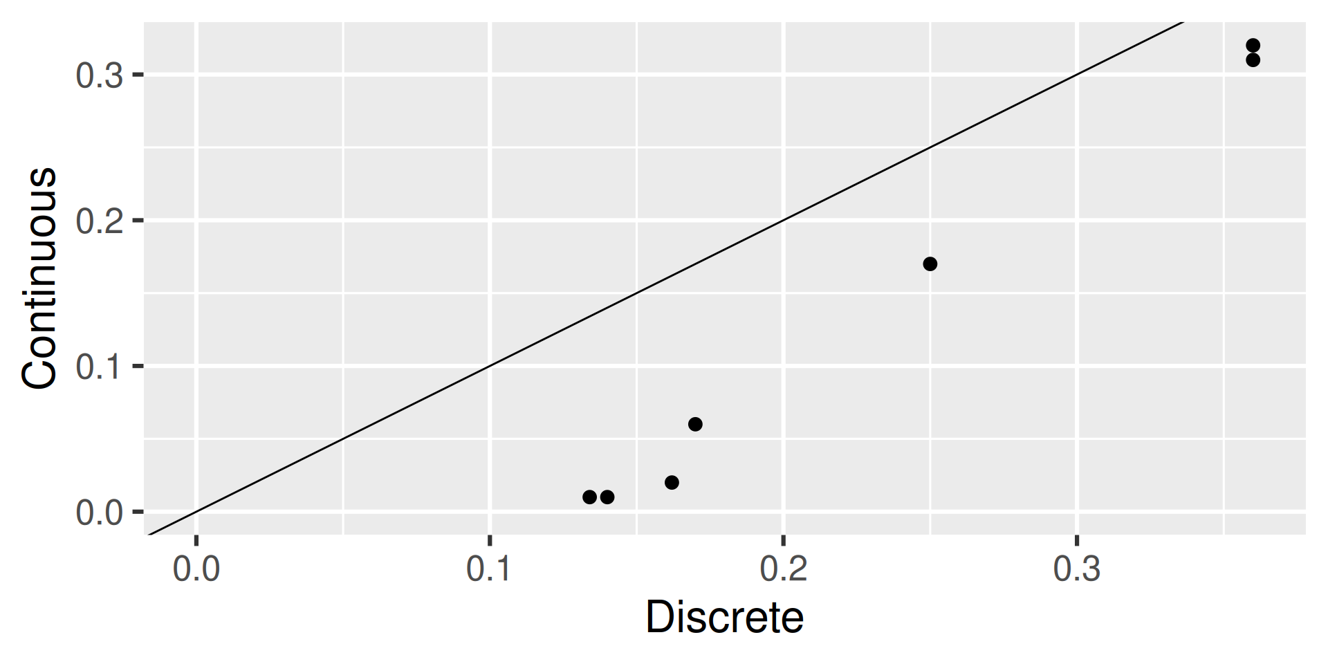
• We now want to join the closest continuous sensor time with the discrete sample time.

• This is trickier than joining by exact matches.

• dplyr has a way, but it’s complicated if you want the absolute closest in either direction

• Another package data.table has a slick way to get the closest matches

Workflow 5: Join Discrete and Continuous

library(data.table)
setDT(discrete_data)[, join_date := Activity_StartDateTime]
setDT(continuous_data)[, join_date := dateTime]
  
closest_dt <- continuous_data[discrete_data, on = .(join_date), roll = "nearest"]  
closest_dt <- data.frame(closest_dt)

Workflow 5: Inspect

ggplot(data = closest_dt) +
  geom_point(aes(x = Result_Measure,
                 y = X_99133_00000)) +
  geom_abline() +
  expand_limits(x = 0, y = 0) +
  xlab("Discrete") +
  ylab("Continuous")

Data Discovery

The process for discovering data is a bit in flux with NWIS retiring. I expect a new process will be introduced soon. For now here are some options.

1. read_waterdata_ts_meta discovers daily and continuous time series

2. summarize_waterdata_samples discovers discrete data at specific monitoring locations

The next slides will demo how to use those.

Data Discovery: Time Series

ts_available <- read_waterdata_ts_meta(monitoring_location_id = "USGS-04183500")

Data Discovery: Discrete

discrete_available <- summarize_waterdata_samples(monitoringLocationIdentifier = "USGS-04183500")

characteristicUserSupplied

• characteristicUserSupplied can be an input to read_waterdata_sample

discrete1 <- read_waterdata_samples(characteristicUserSupplied = "Phosphorus as phosphorus, water, unfiltered", 
                                    monitoringLocationIdentifier = "USGS-04183500")
nrow(discrete1)

[1] 1226

More Information

• dataRetrieval repository:
  • https://github.com/DOI-USGS/dataRetrieval
  • Documentation
  • dataRetrieval New Features
  • General Tutorial
• Contact:
  • Computational Tools Email: comptools@usgs.gov