Increasingly there are high frequency sensor data available for water quality data. There’s a need to join the sensor and discrete data by the closest time.
This article will discuss how to do that using the
data.table package.
Let’s look at site “01646500”, and a nearby site with a real-time nitrate-plus-nitrite sensor. Our goal is to get the discharge and nitrate-plus-nitrite sensor data aligned with the discrete water quality samples.
library(dataRetrieval)

site_uv <- "USGS-01646500"
site_samples <- "USGS-01646580"
pcode_uv <- "99133"
pcode_samples <- "00631"
start_date <- as.Date("2018-01-01")
end_date <- as.Date("2020-01-01")

samples_data <- read_waterdata_samples(
  monitoringLocationIdentifier = site_samples,
  usgsPCode = pcode_samples,
  activityStartDateUpper = end_date,
  activityStartDateLower = start_date,
  dataProfile = "fullphyschem")

uv_data <- read_waterdata_continuous(monitoring_location_id = site_uv,
                                     parameter_code =  c(pcode_uv),
                                     time = c(start_date, end_date))
Next we’ll clean up the discrete water quality data to make it easy to follow in this tutorial.
samples_trim <- samples_data |>
  filter(Activity_TypeCode == "Sample-Routine",
         !is.na(Activity_StartDateTime)) |>
  select(samples_date = Activity_StartDateTime,
         val_samples = Result_Measure,
det_txt = Result_ResultDetectionCondition)| samples_date | val_samples | det_txt |
|---|---|---|
| 2018-01-04 15:30:00 | 1.39 | |
| 2018-01-15 15:15:00 | 1.73 | |
| 2018-02-01 15:30:00 | 1.66 | |
| 2018-02-11 19:00:00 | 1.33 | |
| 2018-02-13 17:30:00 | 1.53 | |
| 2018-02-15 16:00:00 | 1.65 |
Finally, we’ll use the data.table package to do a join
to the nearest date. The code to do that is here:
library(data.table)

setDT(samples_trim)[, join_date := samples_date]

setDT(uv_data)[, join_date := time]

closest_dt <- uv_data[samples_trim, on = .(join_date), roll = "nearest"]
closest_dt is a data.table object. It
similar to a data.frame, but not identical. We can convert it to a
data.frame and then use dplyr commands. Note: the whole
analysis can be done via data.table, but most examples in
dataRetrieval have used dplyr, which is why we
bring it back to data.frame. dplyr also has a
join_by(closest()) option, but it is more complicated
because you can only specify the closeness in either the forward or
backwards direction (and we want either direction).
We can calculate “delta_time” - the difference in time between the uv
and samples data. We’ll probably want to add a threshold that we don’t
join values if they are too far apart in time. In this example, if the
difference is greater than 24 hours, we’ll substitute
NA.
samples_closest <- data.frame(closest_dt) |>
  mutate(delta_time = difftime(samples_date, time,
                               units = "hours"),
         val_uv = if_else(abs(as.numeric(delta_time)) >= 24, NA, value)) |>
select(-join_date)| monitoring_location_id | parameter_code | statistic_id | time | value | unit_of_measure | approval_status | last_modified | qualifier | time_series_id | samples_date | val_samples | det_txt | delta_time | val_uv |
|---|---|---|---|---|---|---|---|---|---|---|---|---|---|---|
| USGS-01646500 | 99133 | 00011 | 2018-01-04 15:30:00 | 1.43 | mg/l | Approved | 2025-08-25 23:48:02 | ceea3bb9b349410ba4ad72128cb63392 | 2018-01-04 15:30:00 | 1.39 | 0 hours | 1.43 | ||
| USGS-01646500 | 99133 | 00011 | 2018-01-15 15:15:00 | 1.84 | mg/l | Approved | 2025-08-25 23:48:02 | ceea3bb9b349410ba4ad72128cb63392 | 2018-01-15 15:15:00 | 1.73 | 0 hours | 1.84 | ||
| USGS-01646500 | 99133 | 00011 | 2018-02-01 15:30:00 | 1.67 | mg/l | Approved | 2025-08-25 23:48:02 | ceea3bb9b349410ba4ad72128cb63392 | 2018-02-01 15:30:00 | 1.66 | 0 hours | 1.67 | ||
| USGS-01646500 | 99133 | 00011 | 2018-02-11 19:00:00 | 1.29 | mg/l | Approved | 2025-08-25 23:48:02 | ceea3bb9b349410ba4ad72128cb63392 | 2018-02-11 19:00:00 | 1.33 | 0 hours | 1.29 | ||
| USGS-01646500 | 99133 | 00011 | 2018-02-13 17:30:00 | 1.63 | mg/l | Approved | 2025-08-25 23:48:02 | ceea3bb9b349410ba4ad72128cb63392 | 2018-02-13 17:30:00 | 1.53 | 0 hours | 1.63 | ||
| USGS-01646500 | 99133 | 00011 | 2018-02-15 16:00:00 | 1.68 | mg/l | Approved | 2025-08-25 23:48:02 | ceea3bb9b349410ba4ad72128cb63392 | 2018-02-15 16:00:00 | 1.65 | 0 hours | 1.68 |
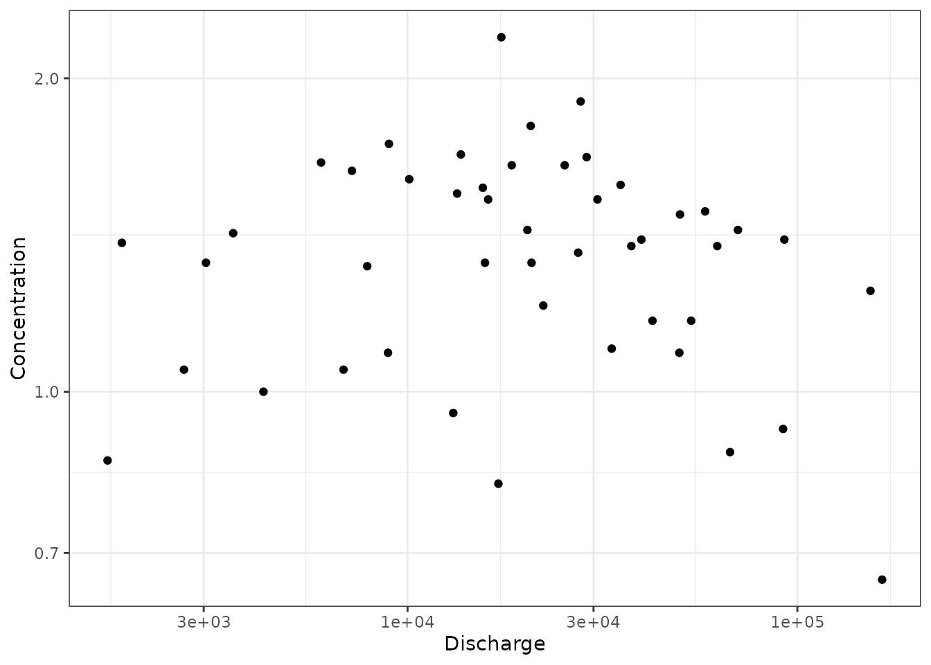
Here are a few plots to show the applications of these joins:
library(ggplot2)

ggplot(data = samples_closest) +
  geom_point(aes(x = val_uv, y = val_samples)) +
  theme_bw() +
  xlab("Sensor") +
  ylab("Discrete")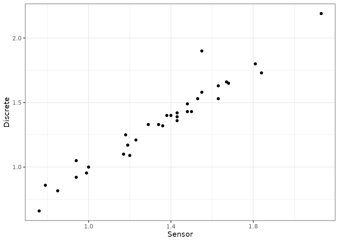
ggplot() +
  geom_line(data = uv_data,
            aes(x = time, value),
            color = "lightgrey") +
  geom_point(data = samples_closest,
             aes(x = samples_date, y = val_samples),
             color= "red") +
  theme_bw() +
  ggtitle("Red dots = discrete samples, grey lines = continuous sensor") +
  xlab("") +
  ylab("Concentration")