Solution Demonstrations for `pycap`

First, make some imports

[1]:

import sys

sys.path.insert(1, "../../")
import matplotlib.pyplot as plt
import numpy as np

Individual Functions

Set some common variables to evaluate. Note that the units here are using SI units. Almost all the functions in this suite are arbitrary provided the units are self-consistent. In other words, if T is provided in m/d, then Q must by in m**3/d and so on.

[2]:

T = 1000  # Transmissivity [m/day]
S = 3e-6  # Storativity [unitless]
dist = 500  # distance [m]
time = np.logspace(0.1, 2.5, 150)  # time [day]
Q = 4000  # pumping rate [m**3/day]

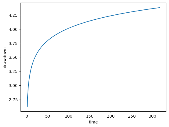
Theis Drawdown

[3]:

from pycap.solutions import theis_drawdown

[4]:

s_theis = theis_drawdown(T, S, time, dist, Q)

[5]:

plt.plot(time, s_theis)
plt.xlabel("time")
plt.ylabel("drawdown")

[5]:

Text(0, 0.5, 'drawdown')

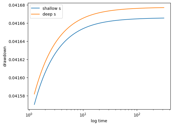
../_images/examples_Solutions_Demonstration_9_1.png

Ward-Lough 2-Layer Drawdown

We need a couple more variables (assuming the previously defined variables pertain to the upper aquifer, then the lower aquifer is defined by T2,S2, etc.) and river and aquitard characterstics.

[6]:

T2 = 1400  # Deep aquifer Transmissivity [m/day]
S2 = 1e-4  # Deep aquifer Storativity [unitless]
width = 10  # stream width [m]
streambed_thick = 20  # stream sediment thickness [m]
streambed_K = 250  # streambed hydraulic conductivity
aquitard_thick = 1  # aquitard thickness [m]
aquitard_K = 50  # aquitard hydraulic conductivity
x = 20  # x-location at which to calculate drawdown
# (x=0 is at the stream)
y = 5  # x-location at which to calculate drawdown
# (y=0 is the along-stream location of the pumping well)

[7]:

from pycap.solutions import ward_lough_drawdown

[8]:

s_wl = ward_lough_drawdown(
    T,
    S,
    time,
    dist,
    Q,
    width=width,
    T2=T2,
    S2=S2,
    streambed_thick=streambed_thick,
    streambed_K=streambed_K,
    aquitard_thick=aquitard_thick,
    aquitard_K=aquitard_K,
    x=x,
    y=y,
)

[9]:

plt.plot(time, s_wl[:, 0], label="shallow s")
plt.plot(time, s_wl[:, 1], label="deep s")
plt.legend()
plt.xscale("log")
plt.xlabel("log time")
plt.ylabel("drawdown")

[9]:

Text(0, 0.5, 'drawdown')

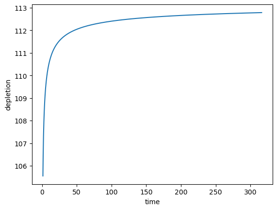
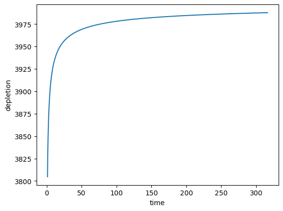
../_images/examples_Solutions_Demonstration_15_1.png

Walton Depletion

Note that this function must use Imperial units of feet for length and days for time.

[10]:

from pycap.solutions import walton_depletion

[11]:

qd = walton_depletion(T * 0.3048, S, time, dist, Q * (0.3048**3))

[12]:

plt.plot(time, qd)
plt.xlabel("time")
plt.ylabel("depletion")

[12]:

Text(0, 0.5, 'depletion')

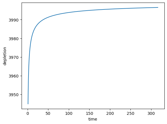
../_images/examples_Solutions_Demonstration_19_1.png

Glover Depletion

[13]:

from pycap.solutions import glover_depletion

[14]:

qd = glover_depletion(T, S, time, dist, Q)

[15]:

plt.plot(time, qd)
plt.xlabel("time")
plt.ylabel("depletion")

[15]:

Text(0, 0.5, 'depletion')

../_images/examples_Solutions_Demonstration_23_1.png

Ward-Lough 2-Layer Depletion

[16]:

from pycap.solutions import ward_lough_depletion

[17]:

qd_wl = ward_lough_depletion(
    T,
    S,
    time,
    dist,
    Q,
    T2=T2,
    S2=S2,
    width=width,
    streambed_thick=streambed_thick,
    streambed_K=streambed_K,
    aquitard_thick=aquitard_thick,
    aquitard_K=aquitard_K,
    x=0,
    y=5,
)

[18]:

plt.plot(time, qd_wl)
plt.xlabel("time")
plt.ylabel("depletion")

[18]:

Text(0, 0.5, 'depletion')

../_images/examples_Solutions_Demonstration_27_1.png

[ ]: