Demonstration of Well Class
Notebook to demonstrate using the Well Class to estimate drawdown or stream depletion using the solutions available in the python module.
[1]:
import sys

sys.path.insert(1, "../../")
import pycap
import matplotlib.pyplot as plt
import numpy as np
import pandas as pd
Example Depletion
The Well class will estimate depletions for streams. The stream distances and streambed conductances, if needed, are passed through dictionaries keyed by a stream name or ID. In this notebook a table of values will be made manually from Table 2 from Reeves, H.W., Hamilton, D.A., Seelbach, P.W., and Asher, A.J., 2009, Ground-water-withdrawal component of the Michigan water-withdrawal screening tool: U.S. Geological Survey Scientific Investigations Report 2009–5003, 36 p.
[https://pubs.usgs.gov/sir/2009/5003/]
pro tip: notice that the distance increases with increasing ID number. Useful for relative reference below.
[2]:
stream_table = pd.DataFrame(
    (
        {"id": 8, "distance": 14802},
        {"id": 9, "distance": 12609.2},
        {"id": 11, "distance": 15750.5},
        {"id": 27, "distance": 22567.6},
        {"id": 9741, "distance": 27565.2},
        {"id": 10532, "distance": 33059.5},
        {"id": 11967, "distance": 14846.3},
        {"id": 12515, "distance": 17042.55},
        {"id": 12573, "distance": 11959.5},
        {"id": 12941, "distance": 19070.8},
        {"id": 13925, "distance": 10028.9},
    )
)
Compute apportionment
The example in the report uses inverse-distance weighting apportionment. Other apportionment approaches that may be used as a simple way to extend the analytical solution are discussed by Zipper and others (2019). [https://agupubs.onlinelibrary.wiley.com/doi/10.1029/2018WR024403]
[3]:
invers = np.array([1 / x for x in stream_table["distance"]])
stream_table["apportionment"] = (1.0 / stream_table["distance"]) / np.sum(invers)
set aquifer properties and streambed conductances
[4]:
T = 7211.0  # ft^2/day
S = 0.01
Q = 70  # 70 gpm --> must convert to cubic feet per day
pumpdays = int(5.0 * 365)
stream_table["conductance"] = 7.11855  # example uses constant streambed_conductance
call a utility to convert Q to a series with appropriate formatting
The Well Class works with a Pandas series of pumping rates, it may be easily constructed with the pycap-dss Q2ts function. The index of the series is pumping days. We also need to convert from pumping in GPM to cubic feet per day so that units are consistent.
[5]:
Q = pycap.Q2ts(pumpdays, 5, Q) * pycap.GPM2CFD
[6]:
Q
[6]:
1       13475.935829
2       13475.935829
3       13475.935829
4       13475.935829
5       13475.935829
            ...
1821    13475.935829
1822    13475.935829
1823    13475.935829
1824    13475.935829
1825    13475.935829
Length: 1825, dtype: float64
[7]:
stream_table.head()
[7]:
| id | distance | apportionment | conductance | |
|---|---|---|---|---|
| 0 | 8 | 14802.0 | 0.098916 | 7.11855 |
| 1 | 9 | 12609.2 | 0.116118 | 7.11855 |
| 2 | 11 | 15750.5 | 0.092959 | 7.11855 |
| 3 | 27 | 22567.6 | 0.064878 | 7.11855 |
| 4 | 9741 | 27565.2 | 0.053116 | 7.11855 |
make dictionaries from the distances, apportionment, and conductance values
[8]:
distances = dict(zip(stream_table.id.values, stream_table.distance.values))
[9]:
apportion = dict(zip(stream_table.id.values, stream_table.apportionment.values))
[10]:
cond = dict(zip(stream_table.id.values, stream_table.conductance.values))
Make a Well object
Depletion and drawdown can be easily returned as attributes of the object. The choice of depletion or drawdown method is made through a parameter passed to the object. In this example the Hunt (1999) depletion method is used to compute stream depletion for the dictionary of streams at the given distances with the inverse-distance apportionment. We also can compute drawdown at a dictionary of locations. If drawdown_dist is not passed to the object, then drawdowns will not be computed. Results are returned as arrays that may easily be converted to Pandas dataframes for ease of viewing and plotting.
[11]:
test_well = pycap.Well(
    T=T,
    S=S,
    Q=Q,
    depletion_years=5,
    depl_method="hunt_99_depletion",
    drawdown_dist={"testlocation0": 50.0},  # default method is Theis
    streambed_conductance=cond,
    stream_dist=distances,
    stream_apportionment=apportion,
)
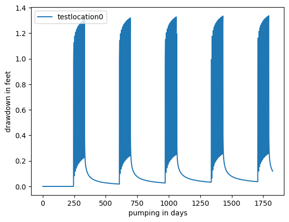
[12]:
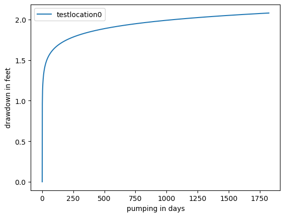
drawdown = pd.DataFrame(test_well.drawdown)
look at drawdown, only one distance was specified. The timeseries is returned however.
[13]:
drawdown.head()
[13]:
| testlocation0 | |
|---|---|
| 0 | 0.000000 |
| 1 | 0.962843 |
| 2 | 1.065859 |
| 3 | 1.126136 |
| 4 | 1.168908 |
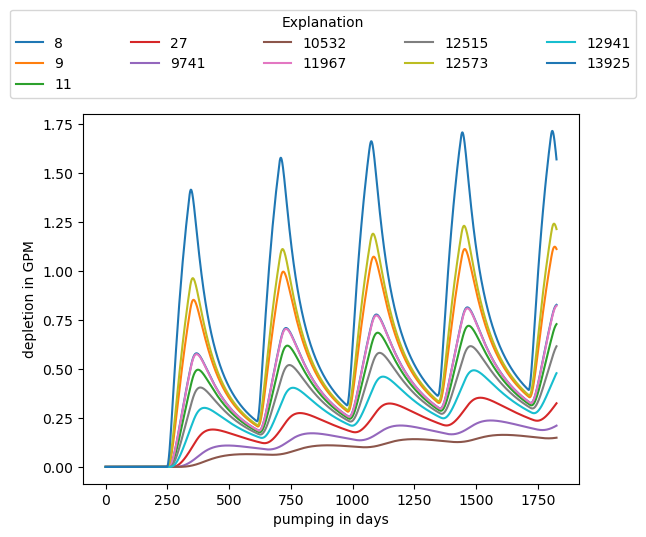
Depletion
The object gives the daily time series according to the pumping schedule. We can pull out the 5-year depletion to note that the final results match Table 2. Note that we need to convert to GPM to compare results to Table 2
[14]:
stream_depl = pd.DataFrame(test_well.depletion)
[15]:
stream_depl = stream_depl * pycap.CFD2GPM
# pull out row for days = 1824 and transpose matrix for ease of comparison to Table 2
five_year = pd.DataFrame(stream_depl.loc[1824].T)
five_year.rename(columns={1824: "Depletion"}, inplace=True)
five_year
[15]:
| Depletion | |
|---|---|
| 8 | 5.144899 |
| 9 | 6.303955 |
| 11 | 4.744429 |
| 27 | 2.869554 |
| 9741 | 2.098081 |
| 10532 | 1.532334 |
| 11967 | 5.125042 |
| 12515 | 4.271490 |
| 12573 | 6.729668 |
| 12941 | 3.660252 |
| 13925 | 8.322122 |
What about plotting?
[16]:
fig, ax = plt.subplots()
drawdown.plot(ax=ax)
ax.set_xlabel("pumping in days")
ax.set_ylabel("drawdown in feet")
[16]:
Text(0, 0.5, 'drawdown in feet')
[17]:
fig, ax = plt.subplots()
stream_depl.plot(ax=ax)
ax.set_xlabel("pumping in days")
ax.set_ylabel("depletion in GPM")
ax.legend(
    title="Explanation",
    bbox_to_anchor=(0, 0.9, 1, 0.9),
    bbox_transform=fig.transFigure,
    ncols=5,
    mode="expand",
    loc="lower left",
)
[17]:
<matplotlib.legend.Legend at 0x1271d07d0>
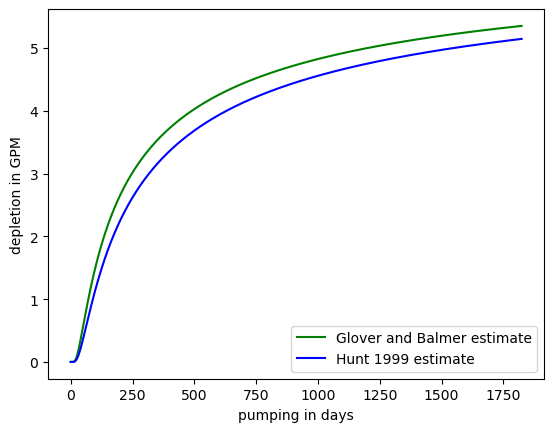
Change depletion method
Several depletion methods are available (see the solutions demonstation notebook for more information). The choice of depletion method is passed to the object as a parameter. Some solutions require additional parameters which need to be passed as named variables.
[18]:
pycap.ALL_DEPL_METHODS
[18]:
{'glover_depletion': <function pycap.solutions.glover_depletion(T, S, time, dist, Q, **kwargs)>,
 'walton_depletion': <function pycap.solutions.walton_depletion(T, S, time, dist, Q, **kwargs)>,
 'hunt_99_depletion': <function pycap.solutions.hunt_99_depletion(T, S, time, dist, Q, streambed_conductance=None, **kwargs)>,
 'hunt_03_depletion': <function pycap.solutions.hunt_03_depletion(T, S, time, dist, Q, Bprime=None, Bdouble=None, aquitard_K=None, sigma=None, width=None, streambed_conductance=None, **kwargs)>,
 'dudley_ward_lough_depletion': <function pycap.solutions.dudley_ward_lough_depletion(T1, S1, time, dist, Q, T2=None, S2=None, width=None, streambed_thick=None, streambed_K=None, aquitard_thick=None, aquitard_K=None, NSteh1=2, **kwargs)>}
[19]:
# for example the Glover and Balmer solution for a stream assuming no streambed resistance. Note that
# the streambed_conductance parameter can be dropped from the call.
test_glover = pycap.Well(
    T=T,
    S=S,
    Q=Q,
    depletion_years=5,
    depl_method="glover_depletion",
    drawdown_dist={"testlocation0": 50.0},  # default method is Theis
    stream_dist=distances,
    stream_apportionment=apportion,
)
[20]:
glover_depl = pd.DataFrame(test_glover.depletion)
glover_depl = glover_depl * pycap.CFD2GPM
[21]:
# plot the two solutions to compare depletion estimates

fig, ax = plt.subplots()
ax.plot(
    glover_depl.index.values,
    glover_depl[8].values,
    "g-",
    label="Glover and Balmer estimate",
)
ax.plot(
    stream_depl.index.values, stream_depl[8].values, "b-", label="Hunt 1999 estimate"
)
ax.set_xlabel("pumping in days")
ax.set_ylabel("depletion in GPM")
ax.legend(loc="lower right")
[21]:
<matplotlib.legend.Legend at 0x127397a10>
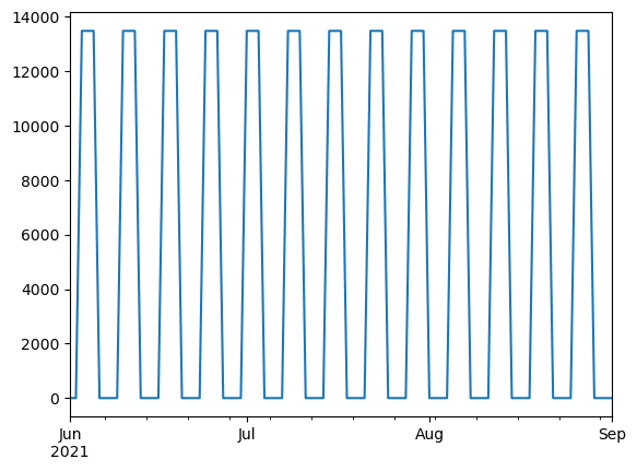
Intermittent Pumping
The Well Class accepts Q as a series of daily pumping rates and will use superposition to produce a timeseries of drawdown or depletion. The Q2ts helper function is one way to generate an input series, but the user can make an arbitrary series.
Set up a series pumping 3 days a week during June, July, and August
[22]:
Q_series = pd.Series(
    index=pd.period_range(start="2020-10-01", end="2025-09-30", freq="D")
)
[23]:
for d in Q_series.index.values:
    Q_series[d] = 0.0
    if d.month in range(6, 9):
        if d.dayofweek in range(3, 6):
            Q_series[d] = 70 * pycap.GPM2CFD
[24]:
fig, ax = plt.subplots()
Q_series.plot(ax=ax)
ax.set_xlim("2021-06-01", "2021-09-01")
[24]:
(18779.0, 18871.0)
Well Class expects series index to be integer days
[25]:
Q_days = pd.Series(Q_series.values, index=range(1, len(Q_series) + 1))
[26]:
Q_days
[26]:
1       0.0
2       0.0
3       0.0
4       0.0
5       0.0
       ...
1822    0.0
1823    0.0
1824    0.0
1825    0.0
1826    0.0
Length: 1826, dtype: float64
[27]:
test_intermittent = pycap.Well(
    T=T,
    S=S,
    Q=Q_days,
    depletion_years=5,
    depl_method="hunt_99_depletion",
    drawdown_dist={"testlocation0": 50.0},  # default method is Theis
    streambed_conductance=cond,
    stream_dist=distances,
    stream_apportionment=apportion,
)
[28]:
intermittent_depl = pd.DataFrame(test_intermittent.depletion) * pycap.CFD2GPM
[29]:
fig, ax = plt.subplots()
intermittent_depl.plot(ax=ax)
ax.set_xlabel("pumping in days")
ax.set_ylabel("depletion in GPM")
ax.legend(
    title="Explanation",
    bbox_to_anchor=(0, 0.9, 1, 0.9),
    bbox_transform=fig.transFigure,
    ncols=5,
    mode="expand",
    loc="lower left",
)
[29]:
<matplotlib.legend.Legend at 0x127399090>
Recall from above that only a single drawdown location was passed to the Well
[30]:
intermittent_drawdown = pd.DataFrame(test_intermittent.drawdown)
[31]:
fig, ax = plt.subplots()
intermittent_drawdown.plot(ax=ax)
ax.set_xlabel("pumping in days")
ax.set_ylabel("drawdown in feet")
ax.legend(loc="upper left")
[31]:
<matplotlib.legend.Legend at 0x12752c090>
Well Class is restricted to Theis drawdown
There are drawdown estimates using the Hunt (1999) and Ward and Lough (2011) solutions; but the Well Class is not currently set up to use these solutions. The user should call the functions directly.
Uncomment the following block and run it to see the error in trying to use other drawdown functions.
[32]:
# test_intermittent = pycap.Well(T=T,
#                  S=S,
#                  Q=Q_days,
#                  depletion_years=5,
#                  depl_method='hunt_99_depletion',
#                  drawdown_dist={'testlocation0':50.},  #default method is Theis
#                  drawdown_method='hunt_99_drawdown',
#                  streambed_conductance=cond,
#                  stream_dist=distances,
#                  stream_apportionment=apportion)
[ ]: