See https://doi-usgs.github.io/EGRET/articles/parallel.html
for an introduction to running in parallel in EGRET. These directions
supplement that article for EGRETci functions.
library(EGRET)
library(EGRETci)
library(parallel)
library(doParallel)

eList <- Choptank_eList
nCores <- detectCores(logical = FALSE) - 2 # leave a core or two out
nCores <- max(c(nCores, 1))
nCores
## [1] 2doParellel
A generalized workflow uses the doParallel package:
cl <- parallel::makeCluster(nCores)
doParallel::registerDoParallel(cl)
eList <- modelEstimation(eList,
                         verbose = FALSE,
                         run.parallel = TRUE)
parallel::stopCluster(cl)
Calculating Confidence Intervals
In series:
nBoot <- 20 # Let's make sure things run with a small nBoot
# but bump up later!

blockLength <- 200

repAnnualResults <- vector(mode = "list", length = nBoot)

for(n in 1:nBoot){
   annualResults <- bootAnnual(eList,
                               blockLength,
                               startSeed = n,
                               verbose = FALSE)
   repAnnualResults[[n]] <- annualResults
}

CIAnnualResults <- ciBands(eList,
                           repAnnualResults)

plotConcHistBoot(eList, CIAnnualResults)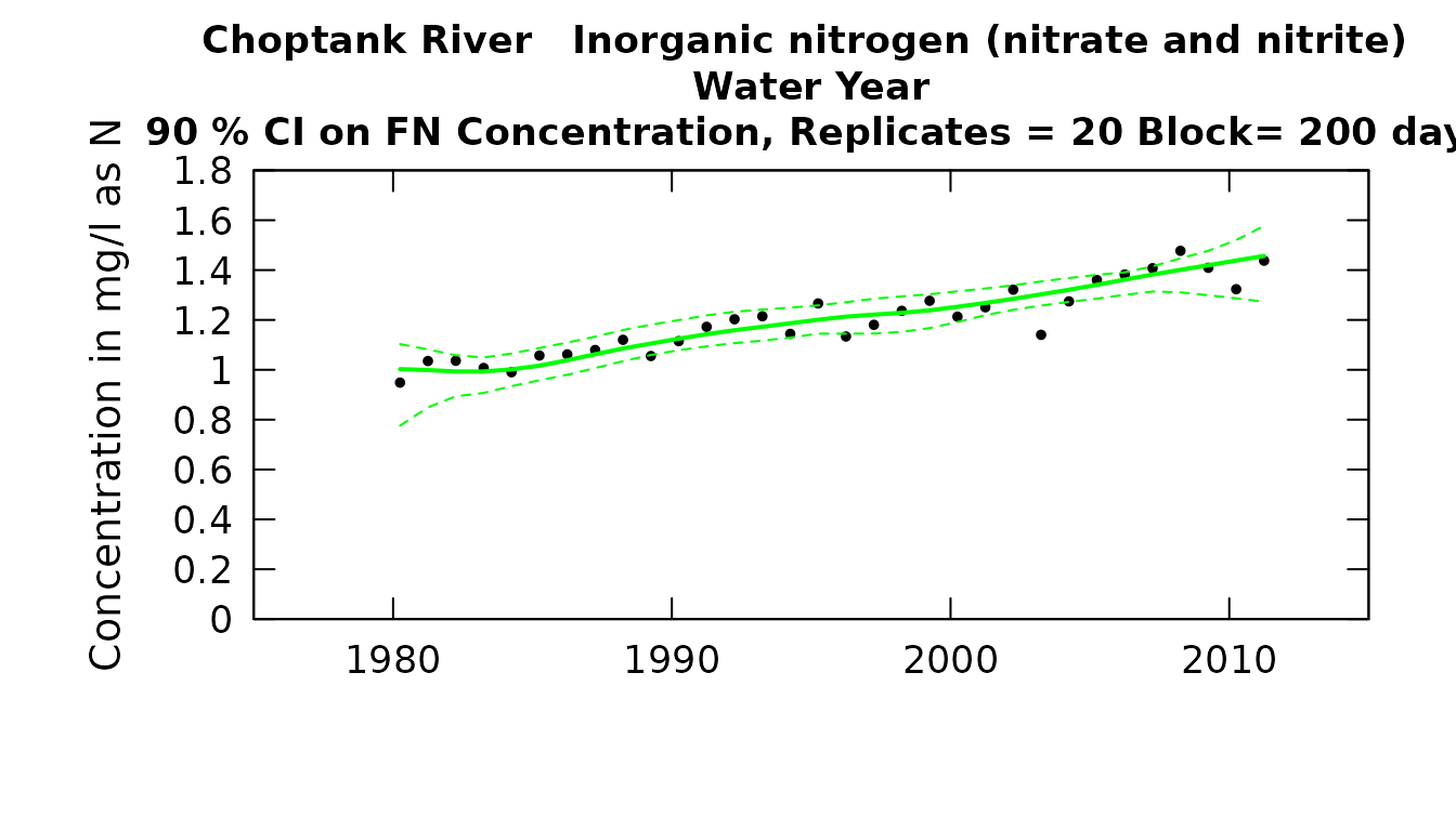
In parallel:
cl <- parallel::makeCluster(nCores)
doParallel::registerDoParallel(cl)
repAnnual <- foreach(n = 1:nBoot,
                     .packages=c('EGRETci', 'EGRET')) %dopar% {
   annualResults <- bootAnnual(eList,
                               blockLength,
                               startSeed = n,
                               verbose = FALSE)
}
parallel::stopCluster(cl)

CIAnnualResults_p <- ciBands(eList, repAnnual)
plotConcHistBoot(eList, CIAnnualResults_p)
runPairs
In series
year1 <- 1985
year2 <- 2010

pairOut_2 <- runPairs(eList, year1, year2, windowSide = 11,
                      verbose = FALSE)

boot_pair_out <- runPairsBoot(eList, pairOut_2,
                              nBoot = nBoot)
##
## Choptank River
## Inorganic nitrogen (nitrate and nitrite)
## Water Year
##
## Change estimates are for 2010 minus 1985
##
## Should we reject Ho that Flow Normalized Concentration Trend = 0 ? Reject Ho
## best estimate of change in concentration is 0.407 mg/L
## Lower and Upper 90% CIs 0.2638524 0.5500715
## also 95% CIs 0.2618548 0.5541293
## and 50% CIs 0.3794161 0.4449768
## approximate two-sided p-value for Conc 0.095
## * Note p-value should be considered to be < stated value
## Likelihood that Flow Normalized Concentration is trending up = 0.976 is trending down = 0.0238
## * Note p-value should be considered to be < stated value
##
## Should we reject Ho that Flow Normalized Flux Trend = 0 ? Reject Ho
## best estimate of change in flux is 0.0476 10^6 kg/year
## Lower and Upper 90% CIs 0.02613975 0.06034084
## also 95% CIs 0.02579486 0.06056007
## and 50% CIs 0.04216098 0.05334703
## approximate two-sided p-value for Flux 0.095
## * Note p-value should be considered to be < stated value
## Likelihood that Flow Normalized Flux is trending up = 0.976 is trending down = 0.0238
##
## Upward trend in concentration is highly likely
## Upward trend in flux is highly likely
## Downward trend in concentration is highly unlikely
## Downward trend in flux is highly unlikely
plotHistogramTrend(eList = eList, eBoot = boot_pair_out,
                   xMin = -5, xMax = 60, xStep = 5,
                   caseSetUp = NA)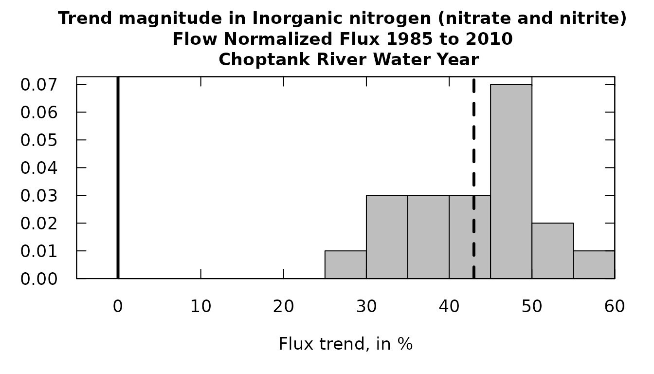
In parallel:
cl <- parallel::makeCluster(nCores)
doParallel::registerDoParallel(cl)

boot_pair_out <- runPairsBoot(eList, pairOut_2,
                              nBoot = nBoot,
                              run.parallel = TRUE)
##
## Choptank River
## Inorganic nitrogen (nitrate and nitrite)
## Water Year
##
## Change estimates are for 2010 minus 1985
##
## Should we reject Ho that Flow Normalized Concentration Trend = 0 ? Reject Ho
## best estimate of change in concentration is 0.407 mg/L
## Lower and Upper 90% CIs 0.2638524 0.5500715
## also 95% CIs 0.2618548 0.5541293
## and 50% CIs 0.3794161 0.4449768
## approximate two-sided p-value for Conc 0.095
## * Note p-value should be considered to be < stated value
## Likelihood that Flow Normalized Concentration is trending up = 0.976 is trending down = 0.0238
## * Note p-value should be considered to be < stated value
##
## Should we reject Ho that Flow Normalized Flux Trend = 0 ? Reject Ho
## best estimate of change in flux is 0.0476 10^6 kg/year
## Lower and Upper 90% CIs 0.02613975 0.06034084
## also 95% CIs 0.02579486 0.06056007
## and 50% CIs 0.04216098 0.05334703
## approximate two-sided p-value for Flux 0.095
## * Note p-value should be considered to be < stated value
## Likelihood that Flow Normalized Flux is trending up = 0.976 is trending down = 0.0238
##
## Upward trend in concentration is highly likely
## Upward trend in flux is highly likely
## Downward trend in concentration is highly unlikely
## Downward trend in flux is highly unlikely
parallel::stopCluster(cl)
plotHistogramTrend(eList = eList,
                   eBoot = boot_pair_out,
                   xMin = -5, xMax = 60, xStep = 5,
                   caseSetUp = NA)
runPairs
In series
groupResults <- runGroups(eList,
                          group1firstYear = 1995,
                          group1lastYear = 2004,
                          group2firstYear = 2005,
                          group2lastYear = 2014,
                          windowSide = 7, wall = TRUE,
                          sample1EndDate = "2004-10-30",
                          paStart = 4, paLong = 2,
                          verbose = FALSE)

boot_group_out <- runGroupsBoot(eList,
                               groupResults,
                               nBoot = nBoot)
##
## Choptank River
## Inorganic nitrogen (nitrate and nitrite)
## Water Year
##
## Change estimates for
## average of 2005 through 2014 minus average of 1995 through 2004
##
## Sample data set was partitioned with a wall at 2004-10-30
##
##
##
## Should we reject Ho that Flow Normalized Concentration Trend = 0 ? Do Not Reject Ho
## best estimate of change in concentration is 0.14 mg/L
## Lower and Upper 90% CIs -0.02781042 0.2736867
## also 95% CIs -0.03034285 0.2769872
## and 50% CIs 0.06160802 0.1766152
## approximate two-sided p-value for Conc 0.15
## Likelihood that Flow Normalized Concentration is trending up = 0.929 is trending down = 0.0714
##
## Should we reject Ho that Flow Normalized Flux Trend = 0 ? Do Not Reject Ho
## best estimate of change in flux is 0.00633 10^6 kg/year
## Lower and Upper 90% CIs -0.01921529 0.02798884
## also 95% CIs -0.0192818 0.02845885
## and 50% CIs -0.004490214 0.01258011
## approximate two-sided p-value for Flux 0.73
## Likelihood that Flow Normalized Flux is trending up = 0.643 is trending down = 0.357
##
## Upward trend in concentration is very likely
## Upward trend in flux is about as likely as not
## Downward trend in concentration is very unlikely
## Downward trend in flux is about as likely as notIn parallel:
cl <- parallel::makeCluster(nCores)
doParallel::registerDoParallel(cl)

boot_group_out <- runGroupsBoot(eList = eList,
                                groupResults = groupResults,
                                nBoot = nBoot,
                                run.parallel = TRUE)
##
## Choptank River
## Inorganic nitrogen (nitrate and nitrite)
## Water Year
##
## Change estimates for
## average of 2005 through 2014 minus average of 1995 through 2004
##
## Sample data set was partitioned with a wall at 2004-10-30
##
##
##
## Should we reject Ho that Flow Normalized Concentration Trend = 0 ? Do Not Reject Ho
## best estimate of change in concentration is 0.14 mg/L
## Lower and Upper 90% CIs -0.02781042 0.2736867
## also 95% CIs -0.03034285 0.2769872
## and 50% CIs 0.06160802 0.1766152
## approximate two-sided p-value for Conc 0.15
## Likelihood that Flow Normalized Concentration is trending up = 0.929 is trending down = 0.0714
##
## Should we reject Ho that Flow Normalized Flux Trend = 0 ? Do Not Reject Ho
## best estimate of change in flux is 0.00633 10^6 kg/year
## Lower and Upper 90% CIs -0.01921529 0.02798884
## also 95% CIs -0.0192818 0.02845885
## and 50% CIs -0.004490214 0.01258011
## approximate two-sided p-value for Flux 0.73
## Likelihood that Flow Normalized Flux is trending up = 0.643 is trending down = 0.357
##
## Upward trend in concentration is very likely
## Upward trend in flux is about as likely as not
## Downward trend in concentration is very unlikely
## Downward trend in flux is about as likely as not
parallel::stopCluster(cl)