
Introducing read_waterdata_statistics_*
Source:vignettes/daily_data_statistics.Rmd
daily_data_statistics.RmdThe read_waterdata_stats_por and
read_waterdata_stats_daterange functions replace the legacy
readNWISstat function. This replacement is necessary
because the legacy API service that readNWISstat uses will
be decommissioned and replaced with a modernized
API. This new API has two available endpoints,
observationNormals and observationIntervals,
that appear similar at first yet have important differences we want to
highlight here.
Fetching day-of-year and month-of-year statistics
Day-of-year and month-of-year statistics aggregate observations for
the same calendar day or month across multiple years to describe typical
seasonal conditions (e.g., all Januarys or all January 1sts). Consider
the output below, where we request day-of-year discharge averages for
January 1 and January 2. Note that the start_date and
end_date are set in month-day format to
describe the day-of-year range.
jan_por_mean <-
  read_waterdata_stats_por(
    monitoring_location_id = site1,
    parameter_code = "00060",
    computation = "arithmetic_mean",
    start_date = "01-01",
    end_date = "01-02"
  )

jan_por_mean
#> Simple feature collection with 3 features and 20 fields
#> Geometry type: POINT
#> Dimension:     XY
#> Bounding box:  xmin: -77.54693 ymin: 37.5632 xmax: -77.54693 ymax: 37.5632
#> Geodetic CRS:  WGS 84
#>   parameter_code unit_of_measure            parent_time_series_id
#> 1          00060          ft^3/s 3995ee5508334084af0a1325f951eadf
#> 2          00060          ft^3/s 3995ee5508334084af0a1325f951eadf
#> 3          00060          ft^3/s 3995ee5508334084af0a1325f951eadf
#>   parent_statistic_id parent_statistic_name time_of_year time_of_year_type
#> 1               00003                  Mean        01-01       day_of_year
#> 2               00003                  Mean        01-02       day_of_year
#> 3               00003                  Mean           01     month_of_year
#>      value sample_count approval_status                       computation_id
#> 1 9342.396           91        approved 9889bbd6-196a-4786-a96a-44110967bb4c
#> 2 9437.714           91        approved 0d2ac9d4-eeac-49e8-8414-6ac0fbb017e1
#> 3 7118.020           91        approved 49c871c5-5cd3-49ff-8d04-e0780876228a
#>       computation percentile monitoring_location_id
#> 1 arithmetic_mean         NA          USGS-02037500
#> 2 arithmetic_mean         NA          USGS-02037500
#> 3 arithmetic_mean         NA          USGS-02037500
#>        monitoring_location_name site_type site_type_code country_code
#> 1 JAMES RIVER NEAR RICHMOND, VA    Stream             ST           US
#> 2 JAMES RIVER NEAR RICHMOND, VA    Stream             ST           US
#> 3 JAMES RIVER NEAR RICHMOND, VA    Stream             ST           US
#>   state_code county_code                  geometry
#> 1         51         087 POINT (-77.54693 37.5632)
#> 2         51         087 POINT (-77.54693 37.5632)
#> 3         51         087 POINT (-77.54693 37.5632)
The first two rows show the average discharge values, aggregated
across all January 1sts and 2nds in the site’s Period of Record (POR).
But wait: what’s in that third row? Looking at the
time_of_year and time_of_year_type columns, we
see the third row represents the average discharge value aggregated
across all Januarys. This illustrates one quirk of the modern
statistics API: any time the start_date to
end_date range overlaps with the first day of a month
(e.g., "01-01"), we will get month-of-year as well as the
day-of-year summary statistics.
You can use the normal_type argument to get only
day-of-year or month-of-year statistics.
read_waterdata_stats_por(
  monitoring_location_id = site1,
  parameter_code = "00060",
  computation = "arithmetic_mean",
  normal_type = "MOY" # or "DOY" for day-of-year
)
#> Simple feature collection with 12 features and 20 fields
#> Geometry type: POINT
#> Dimension:     XY
#> Bounding box:  xmin: -77.54693 ymin: 37.5632 xmax: -77.54693 ymax: 37.5632
#> Geodetic CRS:  WGS 84
#> First 10 features:
#>    parameter_code unit_of_measure            parent_time_series_id
#> 1           00060          ft^3/s 3995ee5508334084af0a1325f951eadf
#> 2           00060          ft^3/s 3995ee5508334084af0a1325f951eadf
#> 3           00060          ft^3/s 3995ee5508334084af0a1325f951eadf
#> 4           00060          ft^3/s 3995ee5508334084af0a1325f951eadf
#> 5           00060          ft^3/s 3995ee5508334084af0a1325f951eadf
#> 6           00060          ft^3/s 3995ee5508334084af0a1325f951eadf
#> 7           00060          ft^3/s 3995ee5508334084af0a1325f951eadf
#> 8           00060          ft^3/s 3995ee5508334084af0a1325f951eadf
#> 9           00060          ft^3/s 3995ee5508334084af0a1325f951eadf
#> 10          00060          ft^3/s 3995ee5508334084af0a1325f951eadf
#>    parent_statistic_id parent_statistic_name time_of_year time_of_year_type
#> 1                00003                  Mean           01     month_of_year
#> 2                00003                  Mean           02     month_of_year
#> 3                00003                  Mean           03     month_of_year
#> 4                00003                  Mean           04     month_of_year
#> 5                00003                  Mean           05     month_of_year
#> 6                00003                  Mean           06     month_of_year
#> 7                00003                  Mean           07     month_of_year
#> 8                00003                  Mean           08     month_of_year
#> 9                00003                  Mean           09     month_of_year
#> 10               00003                  Mean           10     month_of_year
#>      value sample_count approval_status                       computation_id
#> 1  7118.02           91        approved 49c871c5-5cd3-49ff-8d04-e0780876228a
#> 2  8664.40           91        approved bd85b64b-a518-4666-91c9-f8b5901633d6
#> 3  9764.51           91        approved 559696f8-2a14-46a9-85b7-8cecdf3e3dfb
#> 4  8821.21           91        approved afe72737-c2fd-4043-82c9-b0f43a626f95
#> 5  6675.49           91        approved ca7cb19f-b449-494f-ad96-58cce48e0ae6
#> 6  4197.81           91        approved 521201d7-ba6d-4b64-a740-134cbd0c87b6
#> 7  2605.63           91        approved 60d9b482-76db-4357-9d98-74482764b958
#> 8  2298.04           91        approved 22741cd5-a36b-428b-a62b-60cdef6c24d2
#> 9  2009.19           91        approved c29c178d-2d30-467d-8dc2-c1c9417a0303
#> 10 2609.88           92        approved c968af02-a017-490c-a40f-d4dd846c494b
#>        computation percentile monitoring_location_id
#> 1  arithmetic_mean         NA          USGS-02037500
#> 2  arithmetic_mean         NA          USGS-02037500
#> 3  arithmetic_mean         NA          USGS-02037500
#> 4  arithmetic_mean         NA          USGS-02037500
#> 5  arithmetic_mean         NA          USGS-02037500
#> 6  arithmetic_mean         NA          USGS-02037500
#> 7  arithmetic_mean         NA          USGS-02037500
#> 8  arithmetic_mean         NA          USGS-02037500
#> 9  arithmetic_mean         NA          USGS-02037500
#> 10 arithmetic_mean         NA          USGS-02037500
#>         monitoring_location_name site_type site_type_code country_code
#> 1  JAMES RIVER NEAR RICHMOND, VA    Stream             ST           US
#> 2  JAMES RIVER NEAR RICHMOND, VA    Stream             ST           US
#> 3  JAMES RIVER NEAR RICHMOND, VA    Stream             ST           US
#> 4  JAMES RIVER NEAR RICHMOND, VA    Stream             ST           US
#> 5  JAMES RIVER NEAR RICHMOND, VA    Stream             ST           US
#> 6  JAMES RIVER NEAR RICHMOND, VA    Stream             ST           US
#> 7  JAMES RIVER NEAR RICHMOND, VA    Stream             ST           US
#> 8  JAMES RIVER NEAR RICHMOND, VA    Stream             ST           US
#> 9  JAMES RIVER NEAR RICHMOND, VA    Stream             ST           US
#> 10 JAMES RIVER NEAR RICHMOND, VA    Stream             ST           US
#>    state_code county_code                  geometry
#> 1          51         087 POINT (-77.54693 37.5632)
#> 2          51         087 POINT (-77.54693 37.5632)
#> 3          51         087 POINT (-77.54693 37.5632)
#> 4          51         087 POINT (-77.54693 37.5632)
#> 5          51         087 POINT (-77.54693 37.5632)
#> 6          51         087 POINT (-77.54693 37.5632)
#> 7          51         087 POINT (-77.54693 37.5632)
#> 8          51         087 POINT (-77.54693 37.5632)
#> 9          51         087 POINT (-77.54693 37.5632)
#> 10         51         087 POINT (-77.54693 37.5632)
Percentile band plot example
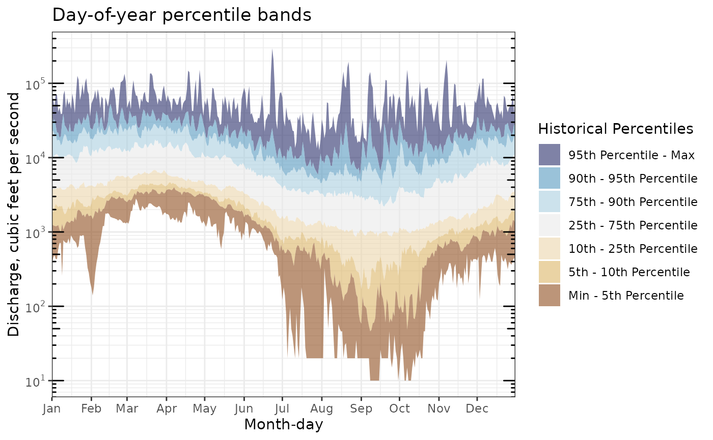
Let’s now look at an example that illustrates the benefits of the statistics API. In the example below, we pull all day-of-year discharge percentiles for our site. Keep in mind that doing so without the statistics API would require us to download the entire daily period of record for this site and hand-compute these percentiles ourselves, a time- and resource-intensive process indeed.
For demonstration, we filter the output to the January 1 day-of-year percentiles, which include a set of percentiles commonly used on the Water Data for the Nation (WDFN) webpages (e.g., Wisconsin water conditions).
full_por_percentiles <-
  read_waterdata_stats_por(
    monitoring_location_id = site1,
    parameter_code = "00060",
    computation = c("minimum", "maximum", "percentile"),
    start_date = "01-01",
    end_date = "12-31"
  )

full_por_percentiles |>
  filter(time_of_year == "01-01" & time_of_year_type == "day_of_year") |>
  arrange(percentile) |>
  select(
    time_of_year,
    computation,
    percentile,
    value
  )
#> Simple feature collection with 9 features and 4 fields
#> Geometry type: POINT
#> Dimension:     XY
#> Bounding box:  xmin: -77.54693 ymin: 37.5632 xmax: -77.54693 ymax: 37.5632
#> Geodetic CRS:  WGS 84
#>   time_of_year computation percentile value                  geometry
#> 1        01-01     minimum          0   380 POINT (-77.54693 37.5632)
#> 2        01-01  percentile          5  1266 POINT (-77.54693 37.5632)
#> 3        01-01  percentile         10  1922 POINT (-77.54693 37.5632)
#> 4        01-01  percentile         25  3580 POINT (-77.54693 37.5632)
#> 5        01-01  percentile         50  5550 POINT (-77.54693 37.5632)
#> 6        01-01  percentile         75  9890 POINT (-77.54693 37.5632)
#> 7        01-01  percentile         90 22000 POINT (-77.54693 37.5632)
#> 8        01-01  percentile         95 37780 POINT (-77.54693 37.5632)
#> 9        01-01     maximum        100 60000 POINT (-77.54693 37.5632)
After a bit of data manipulation, we can then visualize the percentiles as “ribbons” on a plot. Each ribbon spans between two percentiles returned by the /statistics API (e.g., minimum to 5th, 5th to 10th, etc).
doy_perc_bands <-
  full_por_percentiles |>
  sf::st_drop_geometry() |>
  dplyr::filter(time_of_year_type == "day_of_year") |>
  select(time_of_year, percentile, value) |>
  mutate(time_of_year = as.Date(time_of_year, format = "%m-%d")) |>
  pivot_wider(names_from = percentile, values_from = value)

pcode_info <- read_waterdata_parameter_codes(parameter_code = "00060")

bins <- c(
  "95 - Max",
  "90 - 95",
  "75 - 90",
  "25 - 75",
  "10 - 25",
  "5 - 10",
  "Min - 5"
)
bins <- factor(bins, levels = bins)

update_geom_defaults("ribbon", list(alpha = 0.6))

ggplot(data = doy_perc_bands, aes(x = time_of_year)) +
  geom_ribbon(aes(ymin = `95`, ymax = `100`, fill = bins[1])) +
  geom_ribbon(aes(ymin = `90`, ymax = `95`, fill = bins[2])) +
  geom_ribbon(aes(ymin = `75`, ymax = `90`, fill = bins[3])) +
  geom_ribbon(aes(ymin = `25`, ymax = `75`, fill = bins[4])) +
  geom_ribbon(aes(ymin = `10`, ymax = `25`, fill = bins[5])) +
  geom_ribbon(aes(ymin = `5`, ymax = `10`, fill = bins[6])) +
  geom_ribbon(aes(ymin = `0`, ymax = `5`, fill = bins[7])) +
  scale_x_date(
    date_labels = "%b",
    date_breaks = "1 month",
    expand = expand_scale(mult = c(0, 0))
  ) +
  scale_y_log10(
    breaks = scales::breaks_log(base = 10),
    labels = scales::label_log(base = 10),
    minor_breaks = scales::minor_breaks_log()
  ) +
  annotation_logticks(sides = "lr") +
  labs(
    x = "Month-day",
    y = pcode_info$parameter_description,
    title = "Day-of-year percentile bands"
  ) +
  theme_bw() +
  scale_fill_manual(
    "Historical Percentiles",
    values = c(
      "95 - Max" = "#292f6b",
      "90 - 95" = "#5699c0",
      "75 - 90" = "#aacee0",
      "25 - 75" = "#e9e9e9",
      "10 - 25" = "#ebd6ab",
      "5 - 10" = "#dcb668",
      "Min - 5" = "#8f4f1f"
    ),
    labels = c(
      "95th Percentile - Max",
      "90th - 95th Percentile",
      "75th - 90th Percentile",
      "25th - 75th Percentile",
      "10th - 25th Percentile",
      "5th - 10th Percentile",
      "Min - 5th Percentile"
    )
  )
Finally, let’s overlay daily mean data onto the plot:
range <- as.Date(c("2025-01-01", "2026-03-02"))

complete_df <- data.frame(
  time = seq.Date(from = range[1], to = as.Date("2026-12-30"), by = "day")
) |>
  mutate(time_of_year = as.Date(format(time, "%m-%d"), format = "%m-%d"))

daily_data <- complete_df |>
  left_join(
    read_waterdata_daily(
      monitoring_location_id = site1,
      parameter_code = "00060",
      statistic_id = "00003",
      time = range
    ),
    by = "time"
  ) |>
  left_join(doy_perc_bands, by = "time_of_year")

ggplot(data = daily_data, aes(x = time)) +
  geom_ribbon(aes(ymin = `95`, ymax = `100`, fill = bins[1])) +
  geom_ribbon(aes(ymin = `90`, ymax = `95`, fill = bins[2])) +
  geom_ribbon(aes(ymin = `75`, ymax = `90`, fill = bins[3])) +
  geom_ribbon(aes(ymin = `25`, ymax = `75`, fill = bins[4])) +
  geom_ribbon(aes(ymin = `10`, ymax = `25`, fill = bins[5])) +
  geom_ribbon(aes(ymin = `5`, ymax = `10`, fill = bins[6])) +
  geom_ribbon(aes(ymin = `0`, ymax = `5`, fill = bins[7])) +
  geom_line(aes(y = value, color = approval_status), linewidth = 1) +
  scale_x_date(
    date_labels = "%b %Y",
    date_breaks = "3 month",
    expand = expand_scale(mult = c(0, 0))
  ) +
  scale_y_log10(
    breaks = scales::breaks_log(base = 10),
    labels = scales::label_log(base = 10),
    minor_breaks = scales::minor_breaks_log()
  ) +
  annotation_logticks(sides = "lr") +
  scale_color_manual(
    "Status",
    values = c("Approved" = "black", "Provisional" = "red"),
    breaks = c("Approved", "Provisional"),
    limits = force,
    drop = TRUE
  ) +
  scale_fill_manual(
    "Historical Percentiles",
    values = c(
      "95 - Max" = "#292f6b",
      "90 - 95" = "#5699c0",
      "75 - 90" = "#aacee0",
      "25 - 75" = "#e9e9e9",
      "10 - 25" = "#ebd6ab",
      "5 - 10" = "#dcb668",
      "Min - 5" = "#8f4f1f"
    ),
    labels = c(
      "95th Percentile - Max",
      "90th - 95th Percentile",
      "75th - 90th Percentile",
      "25th - 75th Percentile",
      "10th - 25th Percentile",
      "5th - 10th Percentile",
      "Min - 5th Percentile"
    )
  ) +

  labs(
    x = "",
    y = pcode_info$unit_of_measure,
    title = paste0(
      "January 1, 2025 - December 31, 2026\n",
      pcode_info$parameter_description
    )
  ) +
  theme_bw()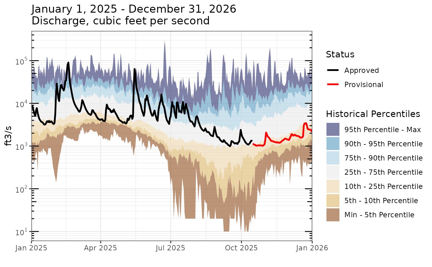
As also seen on the WDFN pages: https://waterdata.usgs.gov/monitoring-location/USGS-02037500/statistical-graphs/
Fetching monthly and annual statistics within a date range
Unlike day- or month-of-year statistics, which summarize typical
seasonal conditions across many years, the
read_waterdata_stats_daterange() function returns summaries
for specific months and years within a requested date range. Consider
the example below where we fetch the average discharge value for the
month of January, 2024. Notice that the start_date and
end_date arguments are given in YYYY-MM-DD
format.
jan_daterange_mean <-
  read_waterdata_stats_daterange(
    monitoring_location_id = site1,
    parameter_code = "00060",
    computation = "arithmetic_mean",
    start_date = "2024-01-01",
    end_date = "2024-01-31"
  )

jan_daterange_mean
#> Simple feature collection with 3 features and 21 fields
#> Geometry type: POINT
#> Dimension:     XY
#> Bounding box:  xmin: -77.54693 ymin: 37.5632 xmax: -77.54693 ymax: 37.5632
#> Geodetic CRS:  WGS 84
#>   parameter_code unit_of_measure            parent_time_series_id
#> 1          00060          ft^3/s 3995ee5508334084af0a1325f951eadf
#> 2          00060          ft^3/s 3995ee5508334084af0a1325f951eadf
#> 3          00060          ft^3/s 3995ee5508334084af0a1325f951eadf
#>   parent_statistic_id parent_statistic_name start_date   end_date interval_type
#> 1               00003                  Mean 2024-01-01 2024-01-31         month
#> 2               00003                  Mean 2024-01-01 2024-12-31 calendar_year
#> 3               00003                  Mean 2023-10-01 2024-09-30    water_year
#>       value sample_count approval_status                       computation_id
#> 1 15787.097           31        approved f8492797-6d92-4c6a-9666-88ec4d1cc8a0
#> 2  6795.699          366        approved e7f9a878-38e8-4984-95d6-3d33a0d498f7
#> 3  6306.902          366        approved ab2893c0-2c2e-4081-b4c2-8e3d2b400382
#>       computation percentile monitoring_location_id
#> 1 arithmetic_mean         NA          USGS-02037500
#> 2 arithmetic_mean         NA          USGS-02037500
#> 3 arithmetic_mean         NA          USGS-02037500
#>        monitoring_location_name site_type site_type_code country_code
#> 1 JAMES RIVER NEAR RICHMOND, VA    Stream             ST           US
#> 2 JAMES RIVER NEAR RICHMOND, VA    Stream             ST           US
#> 3 JAMES RIVER NEAR RICHMOND, VA    Stream             ST           US
#>   state_code county_code                  geometry
#> 1         51         087 POINT (-77.54693 37.5632)
#> 2         51         087 POINT (-77.54693 37.5632)
#> 3         51         087 POINT (-77.54693 37.5632)
Instead of time_of_year and
time_of_year_type columns, this output contains
start_date, end_date, and
interval_type columns representing the daterange over which
the average was calculated. The first row shows the average January,
2024 discharge was about 112 cubic feet per second. We again have extra
rows: the second row contains the calendar year 2024
average and the third contains the water year 2024
average.
Annual statistics will be returned for any calendar/water years than
intersect with the specified date range. Consider the example below,
where the start_date to end_date range is only
93 days yet happens to intersect with calendar and
water years 2023 and 2024. We see this reflected in output containing
monthly averages for September, 2023 through January, 2024 as well as
2023 and 2024 calendar and water year averages.
multiyear_daterange_mean <-
  read_waterdata_stats_daterange(
    monitoring_location_id = site1,
    parameter_code = "00060",
    computation = "arithmetic_mean",
    start_date = "2023-09-30",
    end_date = "2024-01-01"
  )

multiyear_daterange_mean
#> Simple feature collection with 9 features and 21 fields
#> Geometry type: POINT
#> Dimension:     XY
#> Bounding box:  xmin: -77.54693 ymin: 37.5632 xmax: -77.54693 ymax: 37.5632
#> Geodetic CRS:  WGS 84
#>   parameter_code unit_of_measure            parent_time_series_id
#> 1          00060          ft^3/s 3995ee5508334084af0a1325f951eadf
#> 2          00060          ft^3/s 3995ee5508334084af0a1325f951eadf
#> 3          00060          ft^3/s 3995ee5508334084af0a1325f951eadf
#> 4          00060          ft^3/s 3995ee5508334084af0a1325f951eadf
#> 5          00060          ft^3/s 3995ee5508334084af0a1325f951eadf
#> 6          00060          ft^3/s 3995ee5508334084af0a1325f951eadf
#> 7          00060          ft^3/s 3995ee5508334084af0a1325f951eadf
#> 8          00060          ft^3/s 3995ee5508334084af0a1325f951eadf
#> 9          00060          ft^3/s 3995ee5508334084af0a1325f951eadf
#>   parent_statistic_id parent_statistic_name start_date   end_date interval_type
#> 1               00003                  Mean 2023-09-01 2023-09-30         month
#> 2               00003                  Mean 2023-10-01 2023-10-31         month
#> 3               00003                  Mean 2023-11-01 2023-11-30         month
#> 4               00003                  Mean 2023-12-01 2023-12-31         month
#> 5               00003                  Mean 2024-01-01 2024-01-31         month
#> 6               00003                  Mean 2023-01-01 2023-12-31 calendar_year
#> 7               00003                  Mean 2024-01-01 2024-12-31 calendar_year
#> 8               00003                  Mean 2022-10-01 2023-09-30    water_year
#> 9               00003                  Mean 2023-10-01 2024-09-30    water_year
#>       value sample_count approval_status                       computation_id
#> 1  1917.667           30        approved 6cd85fe3-67d9-43e4-aae6-0e76fb8f2778
#> 2  1264.516           31        approved e9e5b782-f8eb-422d-8a56-74c0e5cb1b11
#> 3  2000.333           30        approved 16da6cec-f3c0-428f-bfc0-52790ced9d90
#> 4  5939.355           31        approved 52ac0626-0b21-4b02-b5ad-10dbe891e9d5
#> 5 15787.097           31        approved f8492797-6d92-4c6a-9666-88ec4d1cc8a0
#> 6  5062.219          365        approved 6d659f05-3844-48c0-ae55-2f299dffe792
#> 7  6795.699          366        approved e7f9a878-38e8-4984-95d6-3d33a0d498f7
#> 8  5740.247          365        approved bcfc8a76-36f4-4a8d-86cd-ae8b4e6958d6
#> 9  6306.902          366        approved ab2893c0-2c2e-4081-b4c2-8e3d2b400382
#>       computation percentile monitoring_location_id
#> 1 arithmetic_mean         NA          USGS-02037500
#> 2 arithmetic_mean         NA          USGS-02037500
#> 3 arithmetic_mean         NA          USGS-02037500
#> 4 arithmetic_mean         NA          USGS-02037500
#> 5 arithmetic_mean         NA          USGS-02037500
#> 6 arithmetic_mean         NA          USGS-02037500
#> 7 arithmetic_mean         NA          USGS-02037500
#> 8 arithmetic_mean         NA          USGS-02037500
#> 9 arithmetic_mean         NA          USGS-02037500
#>        monitoring_location_name site_type site_type_code country_code
#> 1 JAMES RIVER NEAR RICHMOND, VA    Stream             ST           US
#> 2 JAMES RIVER NEAR RICHMOND, VA    Stream             ST           US
#> 3 JAMES RIVER NEAR RICHMOND, VA    Stream             ST           US
#> 4 JAMES RIVER NEAR RICHMOND, VA    Stream             ST           US
#> 5 JAMES RIVER NEAR RICHMOND, VA    Stream             ST           US
#> 6 JAMES RIVER NEAR RICHMOND, VA    Stream             ST           US
#> 7 JAMES RIVER NEAR RICHMOND, VA    Stream             ST           US
#> 8 JAMES RIVER NEAR RICHMOND, VA    Stream             ST           US
#> 9 JAMES RIVER NEAR RICHMOND, VA    Stream             ST           US
#>   state_code county_code                  geometry
#> 1         51         087 POINT (-77.54693 37.5632)
#> 2         51         087 POINT (-77.54693 37.5632)
#> 3         51         087 POINT (-77.54693 37.5632)
#> 4         51         087 POINT (-77.54693 37.5632)
#> 5         51         087 POINT (-77.54693 37.5632)
#> 6         51         087 POINT (-77.54693 37.5632)
#> 7         51         087 POINT (-77.54693 37.5632)
#> 8         51         087 POINT (-77.54693 37.5632)
#> 9         51         087 POINT (-77.54693 37.5632)
You can set the interval_type argument to limit the
output to specific intervals.
read_waterdata_stats_daterange(
  monitoring_location_id = site1,
  parameter_code = "00060",
  computation = "arithmetic_mean",
  start_date = "2023-09-30",
  end_date = "2024-01-01",
  interval_type = c("CY", "WY")
)
#> Simple feature collection with 4 features and 21 fields
#> Geometry type: POINT
#> Dimension:     XY
#> Bounding box:  xmin: -77.54693 ymin: 37.5632 xmax: -77.54693 ymax: 37.5632
#> Geodetic CRS:  WGS 84
#>   parameter_code unit_of_measure            parent_time_series_id
#> 1          00060          ft^3/s 3995ee5508334084af0a1325f951eadf
#> 2          00060          ft^3/s 3995ee5508334084af0a1325f951eadf
#> 3          00060          ft^3/s 3995ee5508334084af0a1325f951eadf
#> 4          00060          ft^3/s 3995ee5508334084af0a1325f951eadf
#>   parent_statistic_id parent_statistic_name start_date   end_date interval_type
#> 1               00003                  Mean 2023-01-01 2023-12-31 calendar_year
#> 2               00003                  Mean 2024-01-01 2024-12-31 calendar_year
#> 3               00003                  Mean 2022-10-01 2023-09-30    water_year
#> 4               00003                  Mean 2023-10-01 2024-09-30    water_year
#>      value sample_count approval_status                       computation_id
#> 1 5062.219          365        approved 6d659f05-3844-48c0-ae55-2f299dffe792
#> 2 6795.699          366        approved e7f9a878-38e8-4984-95d6-3d33a0d498f7
#> 3 5740.247          365        approved bcfc8a76-36f4-4a8d-86cd-ae8b4e6958d6
#> 4 6306.902          366        approved ab2893c0-2c2e-4081-b4c2-8e3d2b400382
#>       computation percentile monitoring_location_id
#> 1 arithmetic_mean         NA          USGS-02037500
#> 2 arithmetic_mean         NA          USGS-02037500
#> 3 arithmetic_mean         NA          USGS-02037500
#> 4 arithmetic_mean         NA          USGS-02037500
#>        monitoring_location_name site_type site_type_code country_code
#> 1 JAMES RIVER NEAR RICHMOND, VA    Stream             ST           US
#> 2 JAMES RIVER NEAR RICHMOND, VA    Stream             ST           US
#> 3 JAMES RIVER NEAR RICHMOND, VA    Stream             ST           US
#> 4 JAMES RIVER NEAR RICHMOND, VA    Stream             ST           US
#>   state_code county_code                  geometry
#> 1         51         087 POINT (-77.54693 37.5632)
#> 2         51         087 POINT (-77.54693 37.5632)
#> 3         51         087 POINT (-77.54693 37.5632)
#> 4         51         087 POINT (-77.54693 37.5632)
Monthly average table example
Before we move on, consider the following example where we create a Monthly mean statistics table similar to what you’d find in the Water Year Summaries. Note that the values reported here are slightly different from what you’ll find in the Water Year Summary because of differences in how values are rounded.
monthly_means <-
  read_waterdata_stats_daterange(
    monitoring_location_id = site1,
    parameter_code = "00060",
    computation = "arithmetic_mean"
  ) |>
  dplyr::filter(interval_type == "month") |>
  sf::st_drop_geometry()

monthly_means |>
  filter(start_date >= "2004-10-01" & start_date < "2025-09-01") |>
  mutate(
    Month = lubridate::month(start_date, label = TRUE),
    # reorder based on WY
    Month = factor(Month, month.abb[c(10:12, 1:9)]),
    water_year = lubridate::year(as.Date(start_date) + months(3))
  ) |>
  arrange(Month) |>
  group_by(Month) |>
  summarize(
    `Mean` = round(mean(value), 0),
    `Max (WY)` = paste0(
      round(max(value), 0),
      " (",
      water_year[which.max(value)],
      ")"
    ),
    `Min (WY)` = paste0(
      round(min(value), 0),
      " (",
      water_year[which.min(value)],
      ")"
    ),
    .groups = "drop"
  ) |>
  t() |>
  as.data.frame() |>
  knitr::kable(
    col.names = NULL
)| Month | Oct | Nov | Dec | Jan | Feb | Mar | Apr | May | Jun | Jul | Aug | Sep |
| Mean | 4752 | 6211 | 9464 | 9315 | 11258 | 10980 | 10901 | 10397 | 5855 | 3337 | 2661 | 3370 |
| Max (WY) | 14059 (2019) | 20085 (2019) | 24194 (2019) | 18138 (2010) | 26647 (2025) | 19426 (2019) | 17269 (2019) | 19037 (2020) | 13455 (2013) | 11236 (2013) | 6883 (2020) | 15211 (2018) |
| Min (WY) | 1230 (2009) | 1497 (2008) | 1508 (2018) | 2536 (2018) | 2900 (2009) | 3316 (2017) | 5459 (2025) | 3344 (2006) | 1833 (2008) | 1163 (2010) | 1094 (2008) | 968 (2010) |
Statistics API tips
The statistics API does not follow the same OGC standards as the https://api.waterdata.usgs.gov/ogcapi/v0/ endpoints. This section will focus on important differences between the statistics and OGC-compliant APIs and other tips for working with the endpoint.
Higher API limits: at time of writing, the statistics API is limited to the default limits for any api.gov service which is 4000 requests per hour per IP. The API token used for the other USGS OGC-compliant APIs is included in the request, and changes the limit to 4000 requests per hour per token. There is a chance this could make a difference if you are running code on a shared IP: for example a large office, GitHub, Gitlab, etc.
The API always returns all columns: compared to the OGC-compliant endpoints, which come with
skipGeometryandpropertiesarguments to limit the number of columns returned by the API, there is no way to request a subset of columns from the API.Month-of-year statistics: to return month-of-year statistics using
read_waterdata_stats_por, make sure thestart_datetoend_daterange overlaps with the first day of the month for which you want to data. For example,start_date = "01-01"andend_date = "03-01"will return the month-of-year statistics for January, February, and March (in addition to the day-of-year statistics for each month-day in this range).Monthly and annual statistics: when using
read_waterdata_stats_daterange, the output will return monthly and annual summaries for every calendar month, calendar year, and water year that intersects with thestart_datetoend_daterange. For example,start_date = 2023-12-31andend_date = 2024-10-01will return monthly statistics for each month between December, 2023 through October, 2024 and calendar year statistics for 2023 and 2024 and water year statistics for WY2024 and WY2025.Median comes with percentiles: you never need to set
computation = c("median", "percentile")as the median is returned as the 50th percentile. If you do ask for both median and percentiles, your data set will have two rows containing the median for eachparent_time_series_id.Minimum and maximum do not come with percentiles: minimum and maximum statistics are not returned as percentiles so use
computation = c("minimum", "maximum", "percentile")if you want a “complete” set of order statistics.The API returns specific percentiles: for
computation = "percentile", the API will only ever return the following percentiles: 5th, 10th, 25th, 50th, 75th, 90th, and 95th. If you want other percentiles, you’ll need to pull the daily data period of record usingread_waterdata_dailyand compute them yourself.Pay attention to
sample_count: thesample_countcolumn represents the number of observations used to compute the statistic. As stated in the statistics documentation, there is no minimum requirement for the number of observations to calculate a statistic. This means reported monthly and annual statistics can be based on one daily observation from that month/year. In the case of a single observation, the reportedminimum,maximum,median, andarithmetic_meanwill all be equal to the value of that observation and any other percentiles will beNA.