Introduction to the USGS Water Data APIs

The USGS Water Data APIs are the modern, OGC-based replacement for the legacy NWIS web services. In Python they are exposed through the dataretrieval.waterdata module, which will gradually replace the older dataretrieval.nwis functions.

This notebook tours each new function. The NWIS shut-down timeline is still uncertain, so we recommend migrating to the waterdata functions sooner rather than later.

If you are coming from the R dataRetrieval package, the functions map across as follows:

R `dataRetrieval`	Python `dataretrieval.waterdata`
`read_waterdata_monitoring_location`	`get_monitoring_locations`
`read_waterdata_ts_meta` / `read_waterdata_combined_meta`	`get_time_series_metadata` / `get_combined_metadata`
`read_waterdata_parameter_codes`	`get_reference_table(collection="parameter-codes")`
`read_waterdata_daily`	`get_daily`
`read_waterdata_continuous`	`get_continuous`
`read_waterdata_field_measurements`	`get_field_measurements`
`read_waterdata_channel`	`get_channel`
`read_waterdata_latest_continuous` / `read_waterdata_latest_daily`	`get_latest_continuous` / `get_latest_daily`
`read_waterdata` (CQL)	the `filter` / `filter_lang` arguments on any function
`read_waterdata_metadata`	`get_reference_table`
`read_waterdata_samples`	`get_samples`
`read_waterdata_stats_por` / `read_waterdata_stats_daterange`	`get_stats_por` / `get_stats_date_range`

[1]:

import matplotlib.pyplot as plt
import pandas as pd

from dataretrieval import waterdata

%matplotlib inline
plt.rcParams["figure.figsize"] = (7, 4)

Return values. Every dataretrieval.waterdata function returns a (data, metadata) tuple. The first element is a pandas.DataFrame (or a geopandas.GeoDataFrame when the service returns a geometry column); the second is a small metadata object describing the request. Throughout this notebook we unpack the tuple as df, md = waterdata.get_...(...).

New features

The new API endpoints each deliver a different type of USGS water data, and they all share features the legacy services lacked.

Flexible queries

The new functions expose all of the query parameters the API supports, each defaulting to None. You do not need to (and usually should not) specify them all. Filters are combined with a Boolean AND: passing both a list of monitoring locations and a list of parameter codes returns only the combinations of the two. Because every argument is named, your IDE can autocomplete the options.

Flexible columns returned

Use the properties argument to choose which columns come back. The full set of available properties for a collection is published in that collection’s schema, e.g. https://api.waterdata.usgs.gov/ogcapi/v0/collections/daily/queryables.

[2]:

# Ask for just a few columns instead of the full ~40-column record.
sites_info, _ = waterdata.get_monitoring_locations(
    monitoring_location_id="USGS-01491000",
    properties=[
        "monitoring_location_id",
        "site_type",
        "drainage_area",
        "monitoring_location_name",
    ],
)
sites_info.drop(columns="geometry")

Retrieving: monitoring-locations · 1 page · 1 rows
No API key detected — register for higher rate limits at https://api.waterdata.usgs.gov/signup/

[2]:

	monitoring_location_id	site_type	drainage_area	monitoring_location_name
0	USGS-01491000	Stream	113.0	CHOPTANK RIVER NEAR GREENSBORO, MD

API tokens

USGS now rate-limits requests per IP address per hour. If you hit the limit you can request a free API token at https://api.waterdata.usgs.gov/signup/. Keep it out of shared scripts and version control. (At the time of writing the Python dataretrieval package does not yet wire a token into these calls; the rate limits are generous for the queries below.)

Contextual Query Language (CQL2)

The APIs accept CQL2 expressions for complex queries through the filter / filter_lang arguments. See the General retrieval and CQL2 section below.

Simple features

Spatial collections return a geometry column, so get_* calls give you a geopandas.GeoDataFrame that drops straight into geospatial workflows. Pass skip_geometry=True to get a plain DataFrame.

Lessons learned

Request many sites in one call

dataretrieval automatically splits a large request — many monitoring locations, several parameter codes, or a complex filter — into URL-sized sub-requests and recombines the results, and it can resume a long pull that hits a rate limit or transient server error without refetching completed work. So pass all your sites in one call rather than looping over them.

The main exception is continuous data, which is capped at 3 years per request. See the Continuous Data notebook for large continuous pulls.

New functions

Monitoring location

get_monitoring_locations returns site metadata. To browse the service in a web browser, visit https://api.waterdata.usgs.gov/ogcapi/v0/collections/monitoring-locations.

A simple request for one known USGS site:

[3]:

sites_info, _ = waterdata.get_monitoring_locations(
    monitoring_location_id="USGS-01491000"
)
print(f"{sites_info.shape[1]} columns returned")
sites_info.drop(columns="geometry").T

Retrieving: monitoring-locations · 1 page · 1 rows

44 columns returned

[3]:

	0
monitoring_location_id	USGS-01491000
agency_code	USGS
agency_name	U.S. Geological Survey
monitoring_location_number	01491000
monitoring_location_name	CHOPTANK RIVER NEAR GREENSBORO, MD
district_code	24
country_code	US
country_name	United States of America
state_code	24
state_name	Maryland
county_code	011
county_name	Caroline County
minor_civil_division_code	None
site_type_code	ST
site_type	Stream
hydrologic_unit_code	020600050203
basin_code	None
altitude	2.73
altitude_accuracy	0.1
altitude_method_code	N
altitude_method_name	Interpolated from Digital Elevation Model
vertical_datum	NAVD88
vertical_datum_name	North American Vertical Datum of 1988
horizontal_positional_accuracy_code	S
horizontal_positional_accuracy	Accurate to + or - 1 sec.
horizontal_position_method_code	M
horizontal_position_method_name	Interpolated from MAP.
original_horizontal_datum	NAD83
original_horizontal_datum_name	North American Datum of 1983
drainage_area	113.0
contributing_drainage_area	NaN
time_zone_abbreviation	EST
uses_daylight_savings	Y
construction_date	NaT
aquifer_code	None
national_aquifer_code	None
aquifer_type_code	None
well_constructed_depth	NaN
hole_constructed_depth	NaN
depth_source_code	None
revision_note	WSP 1622: 1948. WDR MD-DE-79-1: 1961(P).
revision_created	2017-11-13T06:00:00+00:00
revision_modified	None

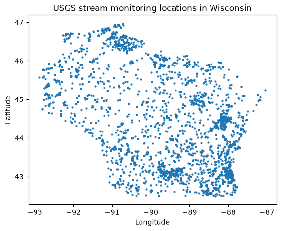
Any returned column can also be used as an input filter. For example, to find every stream site in Wisconsin:

[4]:

sites_wi, _ = waterdata.get_monitoring_locations(
    state_name="Wisconsin",
    site_type="Stream",
)
print(f"{len(sites_wi)} Wisconsin stream sites")
sites_wi[["monitoring_location_id", "monitoring_location_name", "geometry"]].head()

Retrieving: monitoring-locations · 1 page · 2,812 rows

2812 Wisconsin stream sites

[4]:

	monitoring_location_id	monitoring_location_name	geometry
0	ASCE-885512345000005	MLR 2 BATCH TEST - ASCE 005	POINT (-89.13328 44.17978)
1	ASCE-885512345000006	MLR 2 BATCH TEST - ASCE 006	POINT (-89.1725 44.11972)
2	ASCE-885512345000007	MLR 2 BATCH TEST - ASCE 007	POINT (-88.81972 44.09361)
3	USGS-04023120	FLAG RIVER AT PORT WING, WI	POINT (-91.37367 46.78267)
4	USGS-04024025	ST. LOUIS RIVER AT HWY. 23 ABOVE FOND DU LAC, MN	POINT (-92.28408 46.65844)

Because the result is a GeoDataFrame, plotting the locations is a one-liner. For an interactive map, folium works well with the same data.

[5]:

ax = sites_wi.plot(markersize=4, figsize=(7, 5))
ax.set_title("USGS stream monitoring locations in Wisconsin")
ax.set_xlabel("Longitude")
ax.set_ylabel("Latitude")
plt.show()

../_images/examples_USGS_WaterData_Introduction_Examples_12_0.png

Time series & combined metadata

get_combined_metadata joins the monitoring-location catalog (get_monitoring_locations) with the time-series metadata (get_time_series_metadata), returning one row per available time series with both the site attributes and the series’ period of record — a convenient “what data is available” view.

[6]:

ts_available, _ = waterdata.get_combined_metadata(
    monitoring_location_id="USGS-01491000",
    parameter_code=["00060", "00010"],
)
cols = ["parameter_name", "statistic_id", "begin", "end", "last_modified"]
ts_available[cols]

Retrieving: combined-metadata · 1 page · 11 rows

[6]:

	parameter_name	statistic_id	begin	end	last_modified
0	Discharge	NaN	1948-01-15 13:00:00+00:00	2026-06-02 16:17:48+00:00	2026-06-11 18:01:22.547297+00:00
1	Discharge	NaN	1948-01-14 05:00:00+00:00	2025-04-13 04:00:00+00:00	2026-06-03 19:48:05.775076+00:00
2	Temperature, water	00011	2023-04-20 22:30:00+00:00	2026-06-15 13:30:00+00:00	2026-06-15 09:36:26.032031+00:00
3	Temperature, water	00002	2023-04-21 04:00:00+00:00	2026-06-13 04:00:00+00:00	2026-06-15 05:36:31.927264+00:00
4	Discharge	00003	1948-01-01 05:00:00+00:00	2026-06-14 04:00:00+00:00	2026-06-15 05:29:36.160890+00:00
5	Temperature, water	00001	2023-04-21 04:00:00+00:00	2026-06-13 04:00:00+00:00	2026-06-15 05:36:31.529641+00:00
6	Temperature, water	00003	2023-04-21 04:00:00+00:00	2026-06-14 04:00:00+00:00	2026-06-15 05:36:29.741320+00:00
7	Discharge	00011	1990-10-01 09:08:09+00:00	2026-06-15 14:15:00+00:00	2026-06-15 10:27:54.282402+00:00
8	Temperature, water	00001	1988-10-01 04:00:00+00:00	2012-05-09 04:00:00+00:00	2020-08-27 16:15:01.888947+00:00
9	Temperature, water	00002	2010-10-01 04:00:00+00:00	2012-05-09 04:00:00+00:00	2020-08-27 16:16:01.630091+00:00
10	Temperature, water	00003	2010-10-01 04:00:00+00:00	2012-05-09 04:00:00+00:00	2020-08-27 16:15:36.763326+00:00

Parameter codes

Parameter-code descriptions come from the parameter-codes reference table:

[7]:

pcode_info, _ = waterdata.get_reference_table(
    collection="parameter-codes",
    query={"id": "00660"},
)
pcode_info.T

Retrieving: parameter-codes · 1 page · 1 rows

[7]:

	0
parameter_code	00660
parameter_name	Orthophosphate, wf
unit_of_measure	mg/l asPO4
parameter_group_code	NUT
parameter_description	Orthophosphate, water, filtered, milligrams pe...
medium	Water
statistical_basis	None
time_basis	None
weight_basis	None
particle_size_basis	None
sample_fraction	Dissolved
temperature_basis	None
epa_equivalence	Not checked

Daily values

get_daily returns daily values. Browse it at https://api.waterdata.usgs.gov/ogcapi/v0/collections/daily.

[8]:

daily_data, _ = waterdata.get_daily(
    monitoring_location_id="USGS-01491000",
    parameter_code=["00060", "00010"],
    statistic_id="00003",
    time=["2023-10-01", "2024-09-30"],
)
daily_data[["time", "parameter_code", "value", "approval_status"]].head()

Retrieving: daily · 1 page · 730 rows

[8]:

	time	parameter_code	value	approval_status
0	2023-10-01	00010	18.3	Approved
1	2023-10-01	00060	61.9	Approved
2	2023-10-02	00060	57.2	Approved
3	2023-10-02	00010	19.0	Approved
4	2023-10-03	00010	19.6	Approved

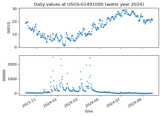
Notice the data come back in long format — one observation per row. Long data are usually easier to work with; here we facet by parameter_code:

[9]:

params = sorted(daily_data["parameter_code"].unique())
fig, axes = plt.subplots(len(params), 1, figsize=(7, 5), sharex=True)
for ax, pcode in zip(axes, params):
    sub = daily_data[daily_data["parameter_code"] == pcode]
    ax.scatter(sub["time"], sub["value"], s=4)
    ax.set_ylabel(pcode)
axes[0].set_title("Daily values at USGS-01491000 (water year 2024)")
axes[-1].set_xlabel("time")
fig.autofmt_xdate()
plt.show()

../_images/examples_USGS_WaterData_Introduction_Examples_20_0.png

Continuous

get_continuous returns instantaneous (sensor) values. Browse it at https://api.waterdata.usgs.gov/ogcapi/v0/collections/continuous.

This service currently allows at most 3 years of data per request; with no time argument it returns the latest year. Continuous data have no geometry column and do not support bounding-box queries. For large pulls, see the Continuous Data notebook.

[10]:

sensor_data, _ = waterdata.get_continuous(
    monitoring_location_id="USGS-01491000",
    parameter_code="00060",
    time="2024-09-01/2024-09-03",
)
sensor_data[["time", "parameter_code", "value", "approval_status"]].head()

Retrieving: continuous · 1 page · 193 rows

[10]:

	time	parameter_code	value	approval_status
0	2024-09-01 00:00:00+00:00	00060	11.7	Approved
1	2024-09-01 00:15:00+00:00	00060	12.0	Approved
2	2024-09-01 00:30:00+00:00	00060	11.7	Approved
3	2024-09-01 00:45:00+00:00	00060	11.7	Approved
4	2024-09-01 01:00:00+00:00	00060	12.0	Approved

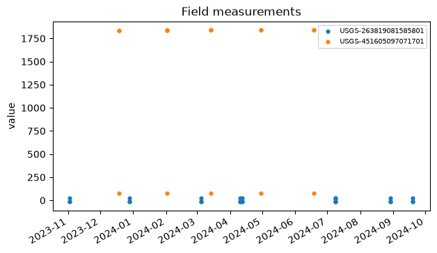
Field measurements

get_field_measurements returns discrete field measurements, including groundwater levels.

[11]:

field_data, _ = waterdata.get_field_measurements(
    monitoring_location_id=[
        "USGS-451605097071701",
        "USGS-263819081585801",
    ],
    time=["2023-10-01", "2024-09-30"],
)
field_data[["time", "monitoring_location_id", "parameter_code", "value"]].head()

Retrieving: field-measurements · 1 page · 42 rows

[11]:

	time	monitoring_location_id	parameter_code	value
0	2023-11-02 18:45:00+00:00	USGS-263819081585801	72019	27.55
1	2023-11-02 18:45:00+00:00	USGS-263819081585801	62610	-14.55
2	2023-11-02 18:45:00+00:00	USGS-263819081585801	62611	-15.68
3	2023-12-18 21:25:00+00:00	USGS-451605097071701	62610	1836.12
4	2023-12-18 21:25:00+00:00	USGS-451605097071701	72019	80.75

[12]:

fig, ax = plt.subplots(figsize=(7, 4))
for site, sub in field_data.groupby("monitoring_location_id"):
    ax.scatter(sub["time"], sub["value"], s=12, label=site)
ax.set_ylabel("value")
ax.set_title("Field measurements")
ax.legend(fontsize=7)
fig.autofmt_xdate()
plt.show()

../_images/examples_USGS_WaterData_Introduction_Examples_25_0.png

Channel measurements

get_channel returns channel-geometry measurements that accompany get_field_measurements.

[13]:

channel, _ = waterdata.get_channel(monitoring_location_id="USGS-02238500")
channel[["time", "channel_width", "channel_area", "channel_velocity"]].head()

Retrieving: channel-measurements · 1 page · 473 rows

[13]:

	time	channel_width	channel_area	channel_velocity
0	1943-02-13 04:00:00+00:00	65.0	306	0.78
1	1943-02-26 04:00:00+00:00	47.0	187	1.07
2	1943-03-30 04:00:00+00:00	58.0	206	0.95
3	1943-05-01 04:00:00+00:00	45.0	200	0.78
4	1943-05-26 04:00:00+00:00	51.0	222	0.85

Latest continuous & latest daily

get_latest_continuous and get_latest_daily have no NWIS equivalent — they return the single most recent observation for each time series.

[14]:

latest_uv, _ = waterdata.get_latest_continuous(
    monitoring_location_id="USGS-01491000",
    parameter_code="00060",
)
cols = ["time", "value", "approval_status", "parameter_code", "unit_of_measure"]
latest_uv[cols].T

Retrieving: latest-continuous · 1 page · 1 rows

[14]:

	0
time	2026-06-15 15:15:00+00:00
value	18.0
approval_status	Provisional
parameter_code	00060
unit_of_measure	ft^3/s

[15]:

latest_dv, _ = waterdata.get_latest_daily(
    monitoring_location_id="USGS-01491000",
    parameter_code="00060",
)
latest_dv[cols].T

Retrieving: latest-daily · 1 page · 1 rows

[15]:

	0
time	2026-06-14 00:00:00
value	17.7
approval_status	Provisional
parameter_code	00060
unit_of_measure	ft^3/s

General retrieval and CQL2

The OGC get_* functions accept a CQL2 expression through the filter / filter_lang arguments, so even complex queries run against these same functions — there is no separate “general retrieval” call.

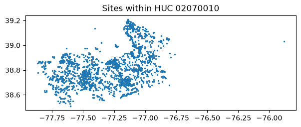
CQL2 supports a wildcard via LIKE (% matches any trailing characters). This is handy for hydrologic unit codes, which may be stored as 02070010 or as a longer code beginning with those digits. To get every site whose HUC starts with 02070010:

[16]:

huc_sites, _ = waterdata.get_monitoring_locations(
    filter="hydrologic_unit_code LIKE '02070010%'",
    filter_lang="cql-text",
)
print(f"{len(huc_sites)} sites in HUC 02070010")
ax = huc_sites.plot(markersize=2, figsize=(7, 5))
ax.set_title("Sites within HUC 02070010")
plt.show()

Retrieving: monitoring-locations · 1 page · 2,354 rows

2354 sites in HUC 02070010

../_images/examples_USGS_WaterData_Introduction_Examples_32_2.png

Numeric filters. Every queryable on the Water Data API is typed as a string, so an unquoted numeric comparison like drainage_area > 1000 is rejected by the server (and quoting it gives a misleading lexicographic comparison). dataretrieval catches this and raises a ValueError:

[17]:

try:
    waterdata.get_monitoring_locations(
        filter="drainage_area > 1000",
        filter_lang="cql-text",
    )
except ValueError as e:
    print(type(e).__name__, "->", str(e)[:120], "...")

ValueError -> Filter uses an unquoted numeric comparison against 'drainage_area' (``drainage_area > 1000``). Every queryable on the Wa ...

The recommended pattern is to filter on the string-valued attributes the server understands (state, site type, HUC, …) and then do the numeric reduction in pandas. For example, large-drainage stream sites in Wisconsin and Minnesota:

[18]:

sites, _ = waterdata.get_monitoring_locations(
    state_name=["Wisconsin", "Minnesota"],
    site_type="Stream",
    properties=[
        "monitoring_location_id",
        "monitoring_location_name",
        "state_name",
        "drainage_area",
    ],
)
big = sites[pd.to_numeric(sites["drainage_area"], errors="coerce") > 1000]
print(f"{len(big)} of {len(sites)} WI/MN stream sites drain > 1000 sq mi")
big.drop(columns="geometry").head()

Retrieving: monitoring-locations · 1 page · 5,399 rows

225 of 5399 WI/MN stream sites drain > 1000 sq mi

[18]:

	monitoring_location_id	monitoring_location_name	state_name	drainage_area
139	USGS-04023500	ST. LOUIS RIVER NEAR CLOQUET, MN	Minnesota	3400.0
141	USGS-04024000	ST. LOUIS RIVER AT SCANLON, MN	Minnesota	3430.0
426	USGS-04062011	BRULE RIVER NEAR COMMONWEALTH, WI	Wisconsin	1020.0
427	USGS-04063000	MENOMINEE RIVER NEAR FLORENCE, WI	Wisconsin	1760.0
456	USGS-04065106	MENOMINEE RIVER AT NIAGARA, WI	Wisconsin	2470.0

Reference tables

get_reference_table exposes a variety of metadata tables. Any returned column can be filtered on. See the USGS Reference Lists notebook for the full list of collections.

Discrete samples

Discrete USGS water-quality data are served from a separate (non-OGC) endpoint via get_samples. See the Discrete water-quality samples notebook.

Daily data statistics

Pre-computed temporal summary statistics are available through get_stats_por (day-of-year / month-of-year) and get_stats_date_range (calendar month, calendar year, water year). See the Daily statistics notebook.

More notes

`limit` and paging

The limit argument sets how many rows come back per page, not the overall total — by default dataretrieval pages through everything. You rarely need to touch it; lowering it can help on a spotty connection.

The `id` column

Each endpoint natively returns an id column, and that value is used as an input to other endpoints under a different name (the monitoring-locations id is the monitoring_location_id everywhere else). dataretrieval renames id accordingly, but you can request the raw id column via properties:

[19]:

site = "USGS-02238500"
renamed, _ = waterdata.get_monitoring_locations(
    monitoring_location_id=site,
    properties=["monitoring_location_id", "state_name", "country_name"],
)
raw_id, _ = waterdata.get_monitoring_locations(
    monitoring_location_id=site,
    properties=["id", "state_name", "country_name"],
)
print("renamed:", [c for c in renamed.columns if c != "geometry"])
print("raw id :", [c for c in raw_id.columns if c != "geometry"])

Retrieving: monitoring-locations · 1 page · 1 rows
Retrieving: monitoring-locations · 1 page · 1 rows

renamed: ['monitoring_location_id', 'state_name', 'country_name']
raw id : ['monitoring_location_id', 'state_name', 'country_name']

More help

Documentation: https://doi-usgs.github.io/dataretrieval-python/
R package docs (source of these examples): https://doi-usgs.github.io/dataRetrieval/
Issues / questions: https://github.com/DOI-USGS/dataretrieval-python/issues