Note
Go to the end to download the full example code.
Frequency domain dataset
import matplotlib.pyplot as plt
from geobipy import CircularLoop
from geobipy import FdemSystem
from geobipy import FdemData
import h5py
import numpy as np
Defining data using a frequency domain system
We can start by defining the frequencies, transmitter loops, and receiver loops For each frequency we need to define a pair of loops
frequencies = np.asarray([395.0, 822.0, 3263.0, 8199.0, 38760.0, 128755.0])
Transmitter positions are defined relative to the observation locations in the data This is usually a constant offset for all data points.
transmitters = CircularLoop(orientation=['z','z','x','z','z','z'],
                             moment=np.r_[1, 1, -1, 1, 1, 1],
                             x = np.r_[0,0,0,0,0,0],
                             y = np.r_[0,0,0,0,0,0],
                             z = np.r_[0,0,0,0,0,0],
                             pitch = np.r_[0,0,0,0,0,0],
                             roll = np.r_[0,0,0,0,0,0],
                             yaw = np.r_[0,0,0,0,0,0],
                             radius = np.r_[1,1,1,1,1,1])
Receiver positions are defined relative to the transmitter
receivers = CircularLoop(orientation=['z','z','x','z','z','z'],
                             moment=np.r_[1, 1, -1, 1, 1, 1],
                             x = np.r_[7.91, 7.91, 9.03, 7.91, 7.91, 7.89],
                             y = np.r_[0,0,0,0,0,0],
                             z = np.r_[0,0,0,0,0,0],
                             pitch = np.r_[0,0,0,0,0,0],
                             roll = np.r_[0,0,0,0,0,0],
                             yaw = np.r_[0,0,0,0,0,0],
                             radius = np.r_[1,1,1,1,1,1])

# Instantiate the system for the data
system = FdemSystem(frequencies=frequencies, transmitter=transmitters, receiver=receivers)

# Create some data with random co-ordinates
x = np.random.randn(100)
y = np.random.randn(100)
z = np.random.randn(100)

data = FdemData(x=x, y=-y, z=z, system = system)
Reading in the Data
Of course measured field data is stored on disk. So instead we can read data from file.
dataFolder = "..//..//supplementary//data//"
# The data file name
dataFile = dataFolder + 'Resolve2.txt'
# The EM system file name
systemFile = dataFolder + 'FdemSystem2.stm'
Read in a data set from file.
FD1 = FdemData.read_csv(dataFile, systemFile)
Take a look at the channel names
for name in FD1.channel_names:
    print(name)

# #%%
# # Get data points by slicing
# FDa = FD1[10:]
# FD1 = FD1[:10]

# #%%
# # Append data sets together
# FD1.append(FDa)


# #%%
# # Plot the locations of the data points
# plt.figure(figsize=(8,6))
# _ = FD1.scatter2D();

# #%%
# # Plot all the data along the specified line
# plt.figure(figsize=(8,6))
# _ = FD1.plotLine(30010.0, log=10);

# #%%
# # Or, plot specific channels in the data
# plt.figure(figsize=(8,6))
# _ = FD1.plot(channels=[0,11,8], log=10, linewidth=0.5);
In_Phase 380.0
In_Phase 1776.0
In_Phase 3345.0
In_Phase 8171.0
In_Phase 41020.0
In_Phase 129550.0
Quadrature 380.0
Quadrature 1776.0
Quadrature 3345.0
Quadrature 8171.0
Quadrature 41020.0
Quadrature 129550.0
Read in a second data set
FD2 = FdemData.read_csv(dataFilename=dataFolder + 'Resolve1.txt', system=dataFolder + 'FdemSystem1.stm')
Warning: Your data contains values that are <= 0.0
We can create maps of the elevations in two separate figures
plt.figure(figsize=(8,6))
_ = FD1.map(dx=50.0, dy=50.0, mask = 200.0)
plt.axis('equal');
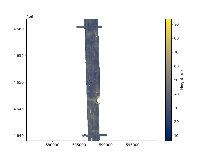
surface [WARNING]: 66659 unusable points were supplied; these will be ignored.
surface [WARNING]: You should have pre-processed the data with block-mean, -median, or -mode.
surface [WARNING]: Check that previous processing steps write results with enough decimals.
surface [WARNING]: Possibly some data were half-way between nodes and subject to IEEE 754 rounding.

(np.float64(584494.28), np.float64(590194.28), np.float64(4639054.24), np.float64(4661854.24))
plt.figure(figsize=(8,6))
_ = FD2.map(dx=50.0, dy=50.0, mask = 200.0)
plt.axis('equal');
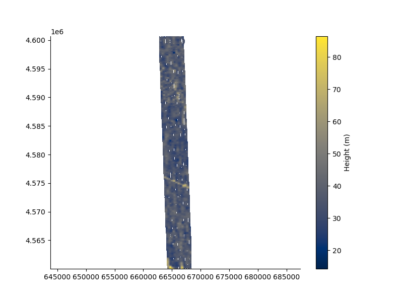
surface [WARNING]: 123487 unusable points were supplied; these will be ignored.
surface [WARNING]: You should have pre-processed the data with block-mean, -median, or -mode.
surface [WARNING]: Check that previous processing steps write results with enough decimals.
surface [WARNING]: Possibly some data were half-way between nodes and subject to IEEE 754 rounding.

(np.float64(662822.398), np.float64(668372.398), np.float64(4560028.655), np.float64(4600678.655))
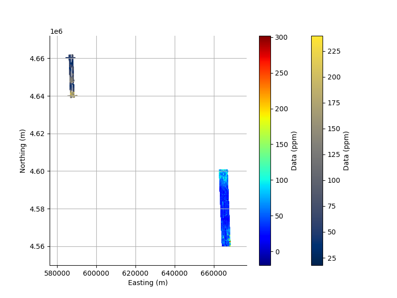
Or, we can plot both data sets in one figure to see their positions relative to each other.
In this case, I use a 2D scatter plot of the data point co-ordinates, and pass one of the channels as the colour.
plt.figure(figsize=(8,6))
_ = FD1.scatter2D(s=1.0, c=FD1.data[:, 0])
_ = FD2.scatter2D(s=1.0, c=FD2.data[:, 0], cmap='jet');
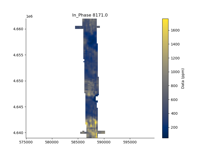
Or, interpolate the values to create a gridded “map”. mapChannel will interpolate the specified channel number.
plt.figure(figsize=(8,6))
_ = FD1.mapData(channel=3, system=0, dx=200, dy=200, mask=250)
plt.axis('equal');
surface [WARNING]: 70336 unusable points were supplied; these will be ignored.
surface [WARNING]: You should have pre-processed the data with block-mean, -median, or -mode.
surface [WARNING]: Check that previous processing steps write results with enough decimals.
surface [WARNING]: Possibly some data were half-way between nodes and subject to IEEE 754 rounding.

(np.float64(584419.28), np.float64(590219.28), np.float64(4638979.24), np.float64(4661979.24))
Export the data to VTK
FD1.to_vtk('FD_one.vtk')
# FD2.to_vtk('FD_two.vtk')
Obtain a line from the data set
Take a look at the line numbers in the dataset
print(np.unique(FD1.lineNumber))
[30010 30020 30030 ... 30100 39010 39020]
L = FD1.line(30010.0)
A summary will now show the properties of the line.
print(L.summary)
FdemData
x:
|   StatArray
|   Name:   Easting (m)
|   Address:['0x153838ed0']
|   Shape:  (6710,)
|   Values: [586852.29 586852.23 586852.17 ... 586123.57 586123.2  586122.82]
|   Min:    586122.82
|   Max:    586852.29
|   has_posterior: False

y:
|   StatArray
|   Name:   Northing (m)
|   Address:['0x15383a2d0']
|   Shape:  (6710,)
|   Values: [4639119.38 4639122.68 4639125.98 ... 4661765.26 4661768.84 4661772.42]
|   Min:    4639119.38
|   Max:    4661772.42
|   has_posterior: False

z:
|   StatArray
|   Name:   Height (m)
|   Address:['0x153838950']
|   Shape:  (6710,)
|   Values: [36.115 36.498 36.835 ... 27.799 27.704 27.601]
|   Min:    23.830000000000002
|   Max:    50.567
|   has_posterior: False

elevation:
|   StatArray
|   Name:   Elevation (m)
|   Address:['0x15383a150']
|   Shape:  (6710,)
|   Values: [1246.84 1246.71 1246.61 ... 1337.94 1337.96 1338.02]
|   Min:    1213.18
|   Max:    1338.02
|   has_posterior: False

channel names:
|   In_Phase 380.0, In_Phase 1776.0, In_Phase 3345.0, In_Phase 8171.0, In_Phase 41020.0,
|   In_Phase 129550.0, Quadrature 380.0, Quadrature 1776.0, Quadrature 3345.0, Quadrature 8171.0,
|   Quadrature 41020.0, Quadrature 129550.0
data:
|   DataArray
|   Name:   Data (ppm)
|   Address:['0x15dc73050']
|   Shape:  (80520,)
|   Values: [145.3 435.8 260.6 ... 749.2 976.5 928.3]
|   Min:    37.7
|   Max:    3726.9

predicted data:
|   DataArray
|   Name:   Predicted Data (ppm)
|   Address:['0x15dc73050']
|   Shape:  (80520,)
|   Values: [0. 0. 0. ... 0. 0. 0.]
|   Min:    0.0
|   Max:    0.0

std:
|   DataArray
|   Name:   std (ppm)
|   Address:['0x155d986d0']
|   Shape:  (80520,)
|   Values: [1.453 4.358 2.606 ... 7.492 9.765 9.283]
|   Min:    0.37700000000000006
|   Max:    37.269

line number:
|   DataArray
|   Name:   Line number
|   Address:['0x15e1a14d0']
|   Shape:  (6710,)
|   Values: [30010. 30010. 30010. ... 30010. 30010. 30010.]
|   Min:    30010.0
|   Max:    30010.0

fiducial:
|   DataArray
|   Name:   Fiducial
|   Address:['0x1530f8650']
|   Shape:  (6710,)
|   Values: [30000 30000 30000 ... 30670 30670 30670]
|   Min:    30000
|   Max:    30670

relative error:
|   DataArray
|   Name:   Relative error (%)
|   Address:['0x15383a750']
|   Shape:  (6710, 1)
|   Values: [[0.01]
|    [0.01]
|    [0.01]
|    ...
|    [0.01]
|    [0.01]
|    [0.01]]
|   Min:    0.01
|   Max:    0.01

additive error:
|   DataArray
|   Name:   Additive error (ppm)
|   Address:['0x153839f50']
|   Shape:  (6710, 1)
|   Values: [[0.]
|    [0.]
|    [0.]
|    ...
|    [0.]
|    [0.]
|    [0.]]
|   Min:    0.0
|   Max:    0.0
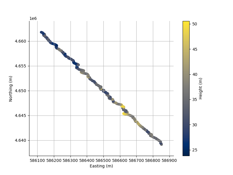
And we can scatter2D the points in the line.
plt.figure(figsize=(8,6))
_ = L.scatter2D();
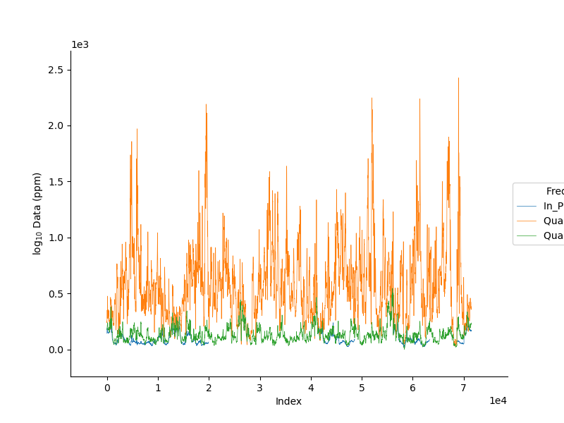
We can specify the axis along which to plot. xAxis can be index, x, y, z, r2d, r3d
plt.figure(figsize=(8,6))
_ = FD1.plot_data(channels=np.r_[0, 11, 8], log=10, linewidth=0.5);

with h5py.File('fdem.h5', 'w') as f:
    FD1.createHdf(f, 'fdem')
    FD1.writeHdf(f, 'fdem')

with h5py.File('fdem.h5', 'r') as f:
    FD3 = FdemData.fromHdf(f['fdem'])

with h5py.File('fdem.h5', 'r') as f:
    fdp = FdemData.fromHdf(f['fdem'], index=0)


# #%%
# # Obtain a single datapoint from the data set
# # +++++++++++++++++++++++++++++++++++++++++++
# #
# # Checkout :ref:`Frequency domain datapoint` for an example
# # about how to use a datapoint once it is instantiated.
# dp = FD1.datapoint(0)

# # Prepare the dataset so that we can read a point at a time.
# Dataset = FdemData._initialize_sequential_reading(dataFile, systemFile)
# # Get a datapoint from the file.
# DataPoint = Dataset._read_record()

plt.show()
File Format for frequency domain data
Here we describe the file format for frequency domain data.
The data columns are read in according to the column names in the first line.
In this description, the column name or its alternatives are given followed by what the name represents. Optional columns are also described.
Required columns
- line
Line number for the data point
- fid
Unique identification number of the data point
- x or northing or n
Northing co-ordinate of the data point, (m)
- y or easting or e
Easting co-ordinate of the data point, (m)
- z or alt
Altitude of the transmitter coil above ground level (m)
- elevation
Elevation of the ground at the data point (m)
- I_<frequency[0]> Q_<frequency[0]> … I_<frequency[last]> Q_<frequency[last]> - with the number and square brackets
The measurements for each frequency specified in the accompanying system file. I is the real inphase measurement in (ppm) Q is the imaginary quadrature measurement in (ppm)
Optional columns
- InphaseErr[0] QuadratureErr[0] … InphaseErr[nFrequencies] QuadratureErr[nFrequencies]
Estimates of standard deviation for each inphase and quadrature measurement. These must appear after the data colums.
Example Header
Line fid easting northing elevation height I_380 Q_380 … … I_129550 Q_129550
File Format for a frequency domain system
The system file is structured using columns with the first line containing header information
Each subsequent row contains the information for each measurement frequency
- freq
Frequency of the channel
- tor
Orientation of the transmitter loop ‘x’, or ‘z’
- tmom
Transmitter moment
- tx, ty, tx
Offset of the transmitter with respect to the observation locations
- ror
Orientation of the receiver loop ‘x’, or ‘z’
- rmom
Receiver moment
- rx, ry, rz
Offset of the receiver with respect to the transmitter location
Example system files are contained in the supplementary folder in this repository
See the Resolve.stm files.
Total running time of the script: (0 minutes 2.933 seconds)