3D Point Cloud class

from geobipy import Point
from os.path import join
import numpy as np
import matplotlib.pyplot as plt
import h5py

nPoints = 200

Create a quick test example using random points $z=x(1-x)cos(4pi x)sin(4pi y^{2})^{2}$

x = -np.abs((2.0 * np.random.rand(nPoints)) - 1.0)
y = -np.abs((2.0 * np.random.rand(nPoints)) - 1.0)
z = x * (1.0 - x) * np.cos(np.pi * x) * np.sin(np.pi * y)

PC3D = Point(x=x, y=y, z=z)

Append pointclouds together

x = np.abs((2.0 * np.random.rand(nPoints)) - 1.0)
y = np.abs((2.0 * np.random.rand(nPoints)) - 1.0)
z = x * (1.0 - x) * np.cos(np.pi * x) * np.sin(np.pi * y)

Other_PC = Point(x=x, y=y, z=z)
PC3D.append(Other_PC)

<geobipy.src.classes.pointcloud.Point.Point object at 0x15d8bd710>

Write a summary of the contents of the point cloud

print(PC3D.summary)

Point
x:
|   StatArray
|   Name:   Easting (m)
|   Address:['0x15e618d50']
|   Shape:  (400,)
|   Values: [-0.71137954 -0.3793497  -0.30956525 ...  0.14065745  0.05106131
|     0.88015259]
|   Min:    -0.9976593326444143
|   Max:    0.9920098541714664
|   has_posterior: False

y:
|   StatArray
|   Name:   Northing (m)
|   Address:['0x15e61a750']
|   Shape:  (400,)
|   Values: [-0.37888241 -0.21170869 -0.82494396 ...  0.71680437  0.78865183
|     0.60356845]
|   Min:    -0.9966527811460972
|   Max:    0.9990626592727034
|   has_posterior: False

z:
|   StatArray
|   Name:   Height (m)
|   Address:['0x15e61b8d0']
|   Shape:  (400,)
|   Values: [-0.6966743   0.11948867  0.11933325 ...  0.08488321  0.02947636
|    -0.09294835]
|   Min:    -1.9925193760132849
|   Max:    0.22842565578586502
|   has_posterior: False

elevation:
|   StatArray
|   Name:   Elevation (m)
|   Address:['0x15e61bad0']
|   Shape:  (400,)
|   Values: [0. 0. 0. ... 0. 0. 0.]
|   Min:    0.0
|   Max:    0.0
|   has_posterior: False

Get a single location from the point as a 3x1 vector

Point = PC3D[50]
# Print the point to the screen

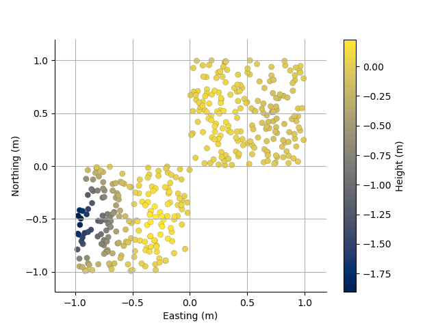
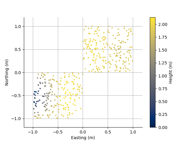
Plot the locations with Height as colour

plt.figure()
PC3D.scatter2D(edgecolor='k')

(<Axes: xlabel='Easting (m)', ylabel='Northing (m)'>, <matplotlib.collections.PathCollection object at 0x15e37bb60>, <matplotlib.colorbar.Colorbar object at 0x15e378050>)

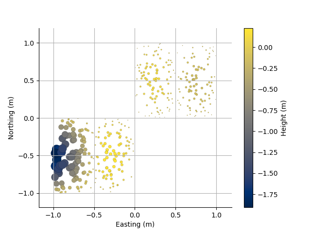
Plotting routines take matplotlib arguments for customization

For example, plotting the size of the points according to the absolute value of height

plt.figure()
ax = PC3D.scatter2D(s=100*np.abs(PC3D.z), edgecolor='k')

Interpolate the points to a 2D rectilinear mesh

mesh, dum = PC3D.interpolate(0.01, 0.01, values=PC3D.z, method='sibson', mask=0.03)

# We can save that mesh to VTK
PC3D.to_vtk('pc3d.vtk')
mesh.to_vtk('interpolated_pc3d.vtk')

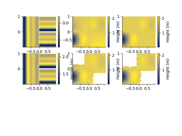
Grid the points using a triangulated CloughTocher, or minimum curvature interpolation

plt.figure()
plt.subplot(331)
PC3D.map(dx=0.01, dy=0.01, method='ct')
plt.subplot(332)
PC3D.map(dx=0.01, dy=0.01, method='mc')
plt.subplot(333)
PC3D.map(dx=0.01, dy=0.01, method='sibson')

plt.subplot(334)
PC3D.map(dx=0.01, dy=0.01, method='ct', mask=0.03)
plt.subplot(335)
PC3D.map(dx=0.01, dy=0.01, method='mc', mask=0.3)
plt.subplot(336)
PC3D.map(dx=0.01, dy=0.01, method='sibson', mask=0.03)

surface [WARNING]: 2 unusable points were supplied; these will be ignored.
surface [WARNING]: You should have pre-processed the data with block-mean, -median, or -mode.
surface [WARNING]: Check that previous processing steps write results with enough decimals.
surface [WARNING]: Possibly some data were half-way between nodes and subject to IEEE 754 rounding.
surface [WARNING]: 2 unusable points were supplied; these will be ignored.
surface [WARNING]: You should have pre-processed the data with block-mean, -median, or -mode.
surface [WARNING]: Check that previous processing steps write results with enough decimals.
surface [WARNING]: Possibly some data were half-way between nodes and subject to IEEE 754 rounding.

(<Axes: >, <matplotlib.collections.QuadMesh object at 0x15e482c00>, <matplotlib.colorbar.Colorbar object at 0x15e898d40>)

For lots of points, these surfaces can look noisy. Using a block filter will help

PCsub = PC3D.block_median(0.05, 0.05)
plt.subplot(337)
PCsub.map(dx=0.01, dy=0.01, method='ct', mask=0.03)
plt.subplot(338)
PCsub.map(dx=0.01, dy=0.01, method='mc', mask=0.03)
plt.subplot(339)
PCsub.map(dx=0.01, dy=0.01, method='sibson', mask=0.03)

surface [WARNING]: 2 unusable points were supplied; these will be ignored.
surface [WARNING]: You should have pre-processed the data with block-mean, -median, or -mode.
surface [WARNING]: Check that previous processing steps write results with enough decimals.
surface [WARNING]: Possibly some data were half-way between nodes and subject to IEEE 754 rounding.

(<Axes: >, <matplotlib.collections.QuadMesh object at 0x15d6e0c20>, <matplotlib.colorbar.Colorbar object at 0x15daf4a70>)

We can perform spatial searches on the 3D point cloud

PC3D.set_kdtree(ndim=2)
p = PC3D.nearest((0.0,0.0), k=200, p=2, radius=0.3)

.nearest returns the distances and indices into the point cloud of the nearest points. We can then obtain those points as another point cloud

# pNear = PC3D[p[1]]
# plt.figure()
# ax1 = plt.subplot(1,2,1)
# pNear.scatter2D()
# plt.plot(0.0, 0.0, 'x')
# plt.subplot(1,2,2, sharex=ax1, sharey=ax1)
# ax, sc, cb = PC3D.scatter2D(edgecolor='k')
# searchRadius = plt.Circle((0.0, 0.0), 0.3, color='b', fill=False)
# ax.add_artist(searchRadius)
# plt.plot(0.0, 0.0, 'x')

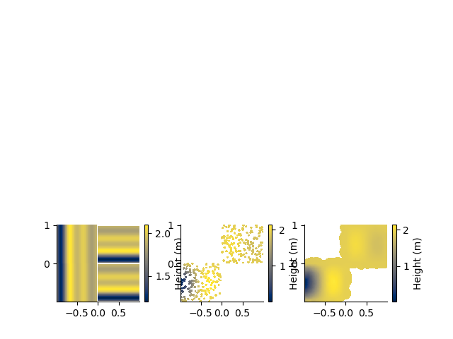
Read in the xyz co-ordinates in columns 2,3,4 from a file. Skip 1 header line.

dataFolder = "..//..//supplementary//Data//"

PC3D.read_csv(filename=dataFolder + 'Resolve1.txt')

<geobipy.src.classes.pointcloud.Point.Point object at 0x15e61e4d0>

plt.figure()
f = PC3D.scatter2D(s=10)

with h5py.File('test.h5', 'w') as f:
    PC3D.createHdf(f, 'test')
    PC3D.writeHdf(f, 'test')

with h5py.File('test.h5', 'r') as f:
    PC3D1 = Point.fromHdf(f['test'])

with h5py.File('test.h5', 'r') as f:
    point = Point.fromHdf(f['test'], index=0)

plt.show()