Frequency domain datapoint

from os.path import join
import numpy as np
import h5py
import matplotlib.pyplot as plt
from geobipy import CircularLoop
from geobipy import FdemSystem
from geobipy import FdemData
from geobipy import FdemDataPoint
from geobipy import RectilinearMesh1D
from geobipy import Model
from geobipy import StatArray
from geobipy import Distribution

# Instantiating a frequency domain data point
# +++++++++++++++++++++++++++++++++++++++++++
#
# To instantiate a frequency domain datapoint we need to define some
# characteristics of the acquisition system.
#
# We need to define the frequencies in Hz of the transmitter,
# and the geometery of the loops used for each frequency.

frequencies = np.asarray([380.0, 1776.0, 3345.0, 8171.0, 41020.0, 129550.0])

# Transmitter positions are defined relative to the observation locations in the data
# This is usually a constant offset for all data points.
transmitters = CircularLoop(orientation=['z','z','x','z','z','z'],
                             moment=np.r_[1, 1, -1, 1, 1, 1],
                             x = np.r_[0,0,0,0,0,0],
                             y = np.r_[0,0,0,0,0,0],
                             z = np.r_[0,0,0,0,0,0],
                             pitch = np.r_[0,0,0,0,0,0],
                             roll = np.r_[0,0,0,0,0,0],
                             yaw = np.r_[0,0,0,0,0,0],
                             radius = np.r_[1,1,1,1,1,1])

# Receiver positions are defined relative to the transmitter
receivers = CircularLoop(orientation=['z','z','x','z','z','z'],
                             moment=np.r_[1, 1, -1, 1, 1, 1],
                             x = np.r_[7.91, 7.91, 9.03, 7.91, 7.91, 7.89],
                             y = np.r_[0,0,0,0,0,0],
                             z = np.r_[0,0,0,0,0,0],
                             pitch = np.r_[0,0,0,0,0,0],
                             roll = np.r_[0,0,0,0,0,0],
                             yaw = np.r_[0,0,0,0,0,0],
                             radius = np.r_[1,1,1,1,1,1])

# Now we can instantiate the system.
fds = FdemSystem(frequencies, transmitters, receivers)

# And use the system to instantiate a datapoint
#
# Note the extra arguments that can be used to create the data point.
# data is for any observed data one might have, while std are the estimated standard
# deviations of those observed data.
#
# Define some in-phase then quadrature data for each frequency.
data = np.r_[145.3, 435.8, 260.6, 875.1, 1502.7, 1516.9,
             217.9, 412.5, 178.7, 516.5, 405.7, 255.7]

fdp = FdemDataPoint(x=0.0, y=0.0, z=30.0, elevation=0.0,
                    data=data, std=None, predictedData=None,
                    system=fds, lineNumber=0.0, fiducial=0.0)

# plt.figure()
# _ = fdp.plot()

# Obtaining a datapoint from a dataset
# ++++++++++++++++++++++++++++++++++++
#
# More often than not, our observed data is stored in a file on disk.
# We can read in a dataset and pull datapoints from it.
#
# For more information about the frequency domain data set see :ref:`Frequency domain dataset`

# Set some paths and file names
dataFolder = "..//..//supplementary//Data//"
# The data file name
dataFile = dataFolder + 'Resolve2.txt'
# The EM system file name
systemFile = dataFolder + 'FdemSystem2.stm'

Initialize and read an EM data set Prepare the dataset so that we can read a point at a time.

Dataset = FdemData._initialize_sequential_reading(dataFile, systemFile)
# Get a datapoint from the file.
fdp = Dataset._read_record()

# # Initialize and read an EM data set
# D = FdemData.read_csv(dataFile,systemFile)

# # Get a data point from the dataset
# fdp = D.datapoint(0)
# plt.figure()
# _ = fdp.plot()

# Using a resolve datapoint
# +++++++++++++++++++++++++

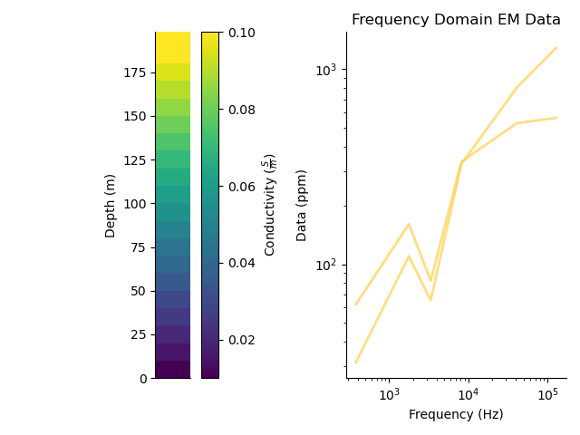
# We can define a 1D layered earth model, and use it to predict some data
nCells = 19
par = StatArray(np.linspace(0.01, 0.1, nCells), "Conductivity", "$\frac{S}{m}$")
depth = StatArray(np.arange(nCells+1) * 10.0, "Depth", 'm')
depth[-1] = np.inf
mod = Model(mesh=RectilinearMesh1D(edges=depth), values=par)

# Forward model the data
fdp.forward(mod)

plt.figure()
plt.subplot(121)
_ = mod.pcolor(transpose=True)
plt.subplot(122)
_ = fdp.plot_predicted()
plt.tight_layout()

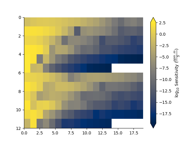
# Compute the sensitivity matrix for a given model
J = fdp.sensitivity(mod)

plt.figure()
_ = np.abs(J).pcolor(equalize=True, log=10, flipY=True)

# Attaching statistical descriptors to the resolve datapoint
# ++++++++++++++++++++++++++++++++++++++++++++++++++++++++++
from numpy.random import Generator
from numpy.random import PCG64DXSM
generator = PCG64DXSM(seed=0)
prng = Generator(generator)

# Set values of relative and additive error for both systems.
fdp.relative_error = 0.05
fdp.additive_error = 10.0
# Define a multivariate log normal distribution as the prior on the predicted data.
fdp.predictedData.prior = Distribution('MvLogNormal', fdp.data[fdp.active], fdp.std[fdp.active]**2.0, prng=prng)

# This allows us to evaluate the likelihood of the predicted data
print(fdp.likelihood(log=True))
# Or the misfit
print(fdp.data_misfit())

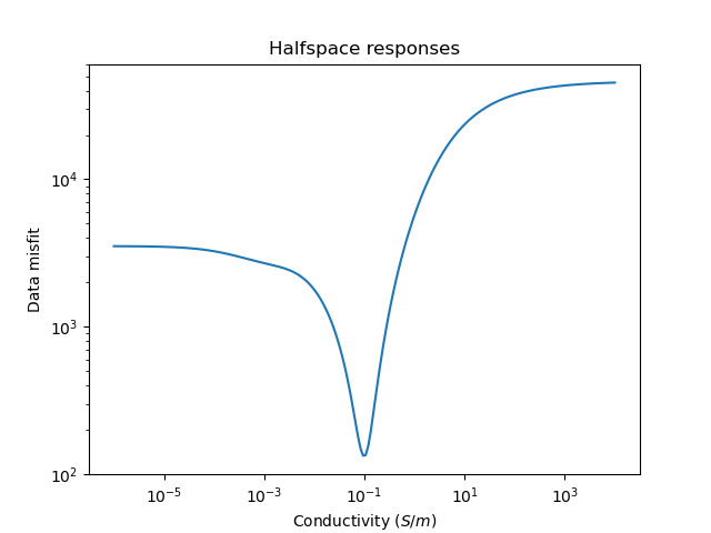
# Plot the misfits for a range of half space conductivities
plt.figure()
_ = fdp.plot_halfspace_responses(-6.0, 4.0, 200)

plt.title("Halfspace responses");

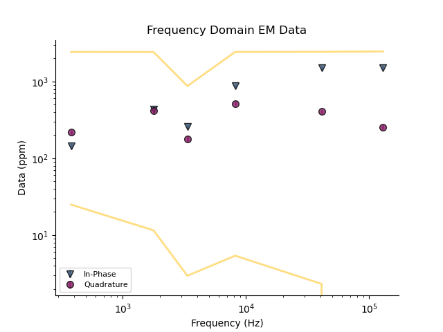
# We can perform a quick search for the best fitting half space
halfspace = fdp.find_best_halfspace()
print('Best half space conductivity is {} $S/m$'.format(halfspace.values))
plt.figure()
_ = fdp.plot()
_ = fdp.plot_predicted()

# Compute the misfit between observed and predicted data
print(fdp.data_misfit())

# We can attach priors to the height of the datapoint,
# the relative error multiplier, and the additive error noise floor


# Define the distributions used as priors.
zPrior = Distribution('Uniform', min=fdp.z - 2.0, max=fdp.z + 2.0, prng=prng)
relativePrior = Distribution('Uniform', min=0.01, max=0.5, prng=prng)
additivePrior = Distribution('Uniform', min=5, max=15, prng=prng)
fdp.set_priors(z_prior=zPrior, relative_error_prior=relativePrior, additive_error_prior=additivePrior, prng=prng)


# In order to perturb our solvable parameters, we need to attach proposal distributions
z_proposal = Distribution('Normal', mean=fdp.z, variance = 0.01, prng=prng)
relativeProposal = Distribution('MvNormal', mean=fdp.relative_error, variance=2.5e-7, prng=prng)
additiveProposal = Distribution('MvLogNormal', mean=fdp.additive_error, variance=1e-4, prng=prng)
fdp.set_proposals(relativeProposal, additiveProposal, z_proposal=z_proposal)

# With priors set we can auto generate the posteriors
fdp.set_posteriors()

nCells = 19
par = StatArray(np.linspace(0.01, 0.1, nCells), "Conductivity", "$\frac{S}{m}$")
depth = StatArray(np.arange(nCells+1) * 10.0, "Depth", 'm')
depth[-1] = np.inf
mod = Model(mesh=RectilinearMesh1D(edges=depth), values=par)
fdp.forward(mod)

# Perturb the datapoint and record the perturbations
for i in range(10):
    fdp.perturb()
    fdp.update_posteriors()


# Plot the posterior distributions
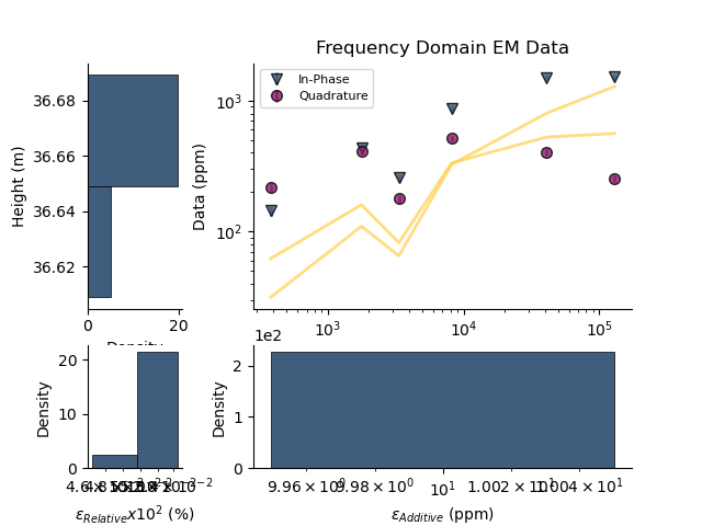
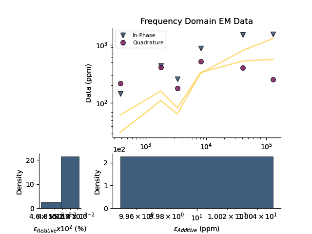
fig = plt.figure()
fdp.plot_posteriors(overlay=fdp)

import h5py
with h5py.File('fdp.h5', 'w') as f:
    fdp.createHdf(f, 'fdp', withPosterior=True)
    fdp.writeHdf(f, 'fdp', withPosterior=True)

with h5py.File('fdp.h5', 'r') as f:
    fdp1 = FdemDataPoint.fromHdf(f['fdp'])

plt.figure()
fdp1.plot_posteriors(overlay=fdp1)

import h5py
with h5py.File('fdp.h5', 'w') as f:
    fdp.createHdf(f, 'fdp', withPosterior=True, add_axis=np.arange(10.0))

    for i in range(10):
        fdp.writeHdf(f, 'fdp', withPosterior=True, index=i)

from geobipy import FdemData
with h5py.File('fdp.h5', 'r') as f:
    fdp1 = FdemDataPoint.fromHdf(f['fdp'], index=0)
    fdp2 = FdemData.fromHdf(f['fdp'])

fdp1.plot_posteriors(overlay=fdp1)

plt.show()
# %%

• 
• 
• 
• 
• 
• 

-733.5454886696688
1367.81945885548
Best half space conductivity is [0.097701] $S/m$
45286.828623928755