Skytem Datapoint Class

Credits: We would like to thank Ross Brodie at Geoscience Australia for his airborne time domain forward modeller https://github.com/GeoscienceAustralia/ga-aem

For ground-based time domain data, we are using Dieter Werthmuller’s python package Empymod https://empymod.github.io/

Thanks to Dieter for his help getting Empymod ready for incorporation into GeoBIPy

from os.path import join
import numpy as np
import h5py
import matplotlib.pyplot as plt
from geobipy import Waveform
from geobipy import SquareLoop, CircularLoop
from geobipy import butterworth
from geobipy import TdemSystem
from geobipy import TdemData
from geobipy import TdemDataPoint
from geobipy import RectilinearMesh1D
from geobipy import Model
from geobipy import StatArray
from geobipy import Distribution

dataFolder = "..//..//supplementary//data//"

# Obtaining a datapoint from a dataset
# ++++++++++++++++++++++++++++++++++++
# More often than not, our observed data is stored in a file on disk.
# We can read in a dataset and pull datapoints from it.
#
# For more information about the time domain data set, see :ref:`Time domain dataset`

# The data file name
dataFile=dataFolder + 'skytem_saline_clay.csv'
# The EM system file name
systemFile=[dataFolder + 'SkytemHM.stm', dataFolder + 'SkytemLM.stm']

Initialize and read an EM data set Prepare the dataset so that we can read a point at a time.

Dataset = TdemData._initialize_sequential_reading(dataFile, systemFile)
# Get a datapoint from the file.
tdp = Dataset._read_record()

Dataset._file.close()

self.n_components=1, self.nTimes=array([26, 19])
self.n_components=1, self.nTimes=array([26, 19])
self.n_components=1, self.nTimes=array([26, 19])
self.n_components=1, self.nTimes=array([26, 19])
self.n_components=1, self.nTimes=array([26, 19])
self.n_components=1, self.nTimes=array([26, 19])
self.n_components=1, self.nTimes=array([26, 19])
self.n_components=1, self.nTimes=array([26, 19])

Using a time domain datapoint

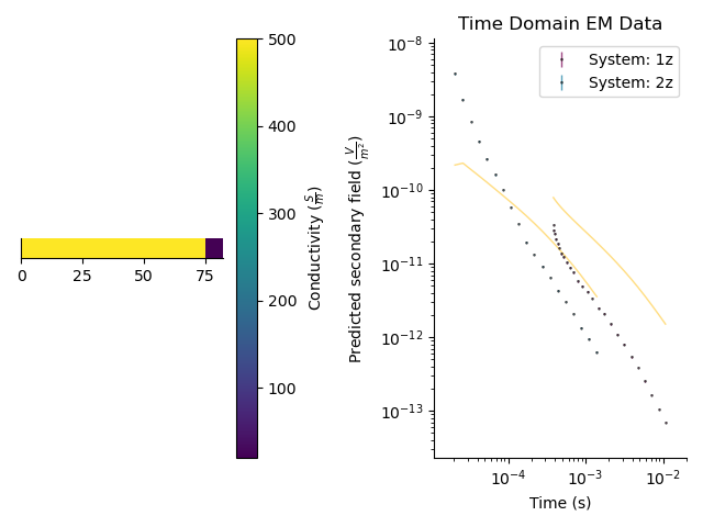
We can define a 1D layered earth model, and use it to predict some data

par = StatArray(np.r_[500.0, 20.0], "Conductivity", "$\frac{S}{m}$")
mod = Model(RectilinearMesh1D(edges=np.r_[0, 75.0, np.inf]), values=par)

Forward model the data

tdp.forward(mod)

plt.figure()
plt.subplot(121)
_ = mod.pcolor()
plt.subplot(122)
_ = tdp.plot()
_ = tdp.plot_predicted()
plt.tight_layout()

/Users/nfoks/codes/repositories/geobipy_docs/geobipy/src/classes/data/datapoint/TdemDataPoint.py:363: RuntimeWarning: divide by zero encountered in log
  additive_error = exp(log(self.additive_error[i]) - 0.5 * (log(off_times) - log(1e-3)))

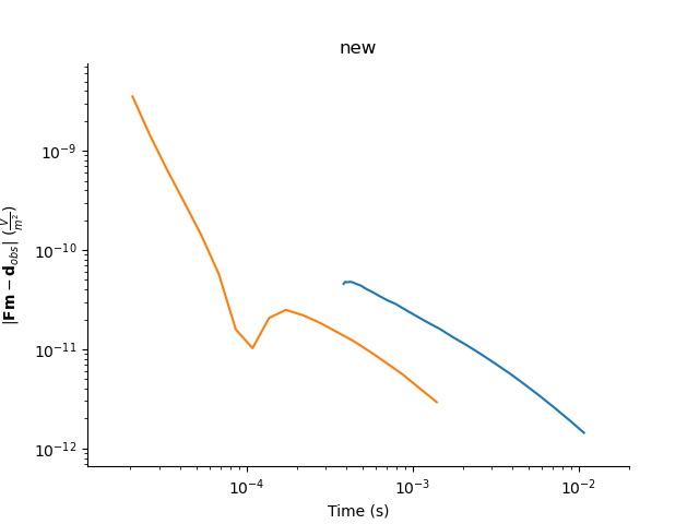
plt.figure()
tdp.plotDataResidual(yscale='log', xscale='log')
plt.title('new')

Text(0.5, 1.0, 'new')

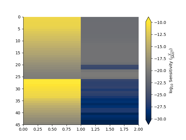
Compute the sensitivity matrix for a given model

J = tdp.sensitivity(mod)
plt.figure()
_ = np.abs(J).pcolor(equalize=True, log=10, flipY=True)

Attaching statistical descriptors to the skytem datapoint

from numpy.random import Generator
from numpy.random import PCG64DXSM
generator = PCG64DXSM(seed=0)
prng = Generator(generator)

# Set values of relative and additive error for both systems.
tdp.relative_error = np.r_[0.05, 0.05]
tdp.additive_error = np.r_[1e-14, 1e-13]
# Define a multivariate normal distribution as the prior on the predicted data.
data_prior = Distribution('MvNormal', tdp.data[tdp.active], tdp.std[tdp.active]**2.0, prng=prng)

tdp.set_priors(data_prior=data_prior)

This allows us to evaluate the likelihood of the predicted data

print(tdp.likelihood(log=True))
# Or the misfit
print(tdp.data_misfit())

-320327.7331520327
643134.8665682999

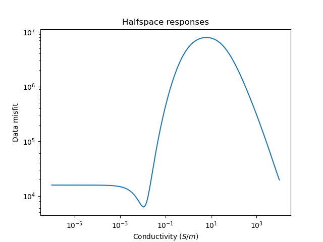
Plot the misfits for a range of half space conductivities

plt.figure()
_ = tdp.plot_halfspace_responses(-6.0, 4.0, 200)
plt.title("Halfspace responses")

Text(0.5, 1.0, 'Halfspace responses')

We can perform a quick search for the best fitting half space

halfspace = tdp.find_best_halfspace()

print('Best half space conductivity is {} $S/m$'.format(halfspace.values))
plt.figure()
_ = tdp.plot()
_ = tdp.plot_predicted()

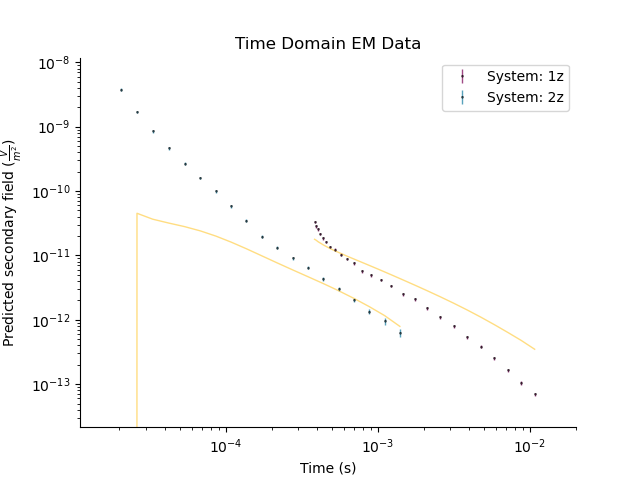
Best half space conductivity is [0.01047616] $S/m$

Compute the misfit between observed and predicted data

print(tdp.data_misfit())

19656.31514467744

We can attach priors to the height of the datapoint, the relative error multiplier, and the additive error noise floor

# Define the distributions used as priors.
z_prior = Distribution('Uniform', min=np.float64(tdp.z) - 2.0, max=np.float64(tdp.z) + 2.0, prng=prng)
relativePrior = Distribution('Uniform', min=np.r_[0.01, 0.01], max=np.r_[0.5, 0.5], prng=prng)
additivePrior = Distribution('Uniform', min=np.r_[1e-16, 1e-16], max=np.r_[1e-10, 1e-10], log=True, prng=prng)
tdp.set_priors(relative_error_prior=relativePrior, additive_error_prior=additivePrior, z_prior=z_prior, prng=prng)

/Users/nfoks/codes/repositories/geobipy_docs/documentation_source/source/examples/Datapoints/plot_skytem_datapoint.py:135: DeprecationWarning: Conversion of an array with ndim > 0 to a scalar is deprecated, and will error in future. Ensure you extract a single element from your array before performing this operation. (Deprecated NumPy 1.25.)
  z_prior = Distribution('Uniform', min=np.float64(tdp.z) - 2.0, max=np.float64(tdp.z) + 2.0, prng=prng)

In order to perturb our solvable parameters, we need to attach proposal distributions

z_proposal = Distribution('Normal', mean=tdp.z, variance = 0.01, prng=prng)
relativeProposal = Distribution('MvNormal', mean=tdp.relative_error, variance=2.5e-7, prng=prng)
additiveProposal = Distribution('MvLogNormal', mean=tdp.additive_error, variance=2.5e-3, linearSpace=True, prng=prng)
tdp.set_proposals(relativeProposal, additiveProposal, z_proposal=z_proposal, prng=prng)

With priorss set we can auto generate the posteriors

tdp.set_posteriors()

Perturb the datapoint and record the perturbations Note we are not using the priors to accept or reject perturbations.

for i in range(10):
    tdp.perturb()
    tdp.update_posteriors()

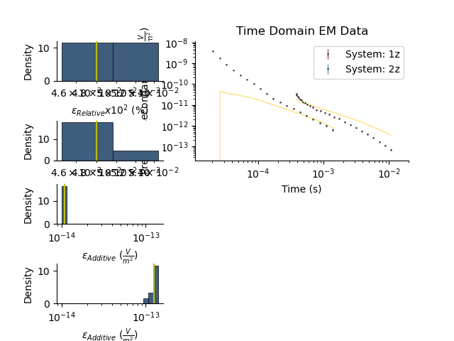
Plot the posterior distributions

plt.figure()
tdp.plot_posteriors(overlay=tdp)

plt.show()

File Format for a time domain datapoint

Here we describe the file format for a time domain datapoint.

For individual datapoints we are using the AarhusInv data format.

Here we take the description for the AarhusInv TEM data file, modified to reflect what we can currently handle in GeoBIPy.

Line 1 :: string

User-defined label describing the TEM datapoint. This line must contain the following, separated by semicolons. XUTM= YUTM= Elevation= StationNumber= LineNumber= Current=

Line 2 :: first integer, sourceType

7 = Rectangular loop source parallel to the x - y plane

Line 2 :: second integer, polarization

3 = Vertical magnetic field

Line 3 :: 6 floats, transmitter and receiver offsets relative to X/Y UTM location.

If sourceType = 7, Position of the center loop sounding.

Line 4 :: Transmitter loop dimensions

If sourceType = 7, 2 floats. Loop side length in the x and y directions

Line 5 :: Fixed

3 3 3

Line 6 :: first integer, transmitter waveform type. Fixed

3 = User defined waveform.

Line 6 :: second integer, number of transmitter waveforms. Fixed

1

Line 7 :: transmitter waveform definition

A user-defined waveform with piecewise linear segments. A full transmitter waveform definition consists of a number of linear segments This line contains an integer as the first entry, which specifies the number of segments, followed by each segment with 4 floats each. The 4 floats per segment are the start and end times, and start and end amplitudes of the waveform. e.g. 3 -8.333e-03 -8.033e-03 0.0 1.0 -8.033e-03 0.0 1.0 1.0 0.0 5.4e-06 1.0 0.0

Line 8 :: On time information. Not used but needs specifying.

1 1 1

Line 9 :: On time low-pass filters. Not used but need specifying.

0

Line 10 :: On time high-pass filters. Not used but need specifying.

0

Line 11 :: Front-gate time. Not used but need specifying.

0.0

Line 12 :: first integer, Number of off time filters

Number of filters

Line 12 :: second integer, Order of the butterworth filter

1 or 2

Line 12 :: cutoff frequencies Hz, one per the number of filters

e.g. 4.5e5

Line 13 :: Off time high pass filters.

See Line 12

Lines after 13 contain 3 columns that pertain to Measurement Time, Data Value, Estimated Standard Deviation

Example data files are contained in the supplementary folder in this repository