1D Model with an infinite halfspace

from copy import deepcopy
from geobipy import StatArray
from geobipy import RectilinearMesh1D
from geobipy import Model
from geobipy import Distribution
import matplotlib.pyplot as plt
import numpy as np

Instantiate the 1D Model with a Half Space

# Make a test model with 10 layers, and increasing parameter values
nLayers = 2
par = StatArray(np.linspace(0.001, 0.02, nLayers), "Conductivity", "$\\frac{S}{m}$")
thk = StatArray(np.full(nLayers, fill_value=10.0))
thk[-1] = np.inf
mesh = RectilinearMesh1D(widths = thk)

mod = Model(mesh = mesh, values=par)

plt.figure()
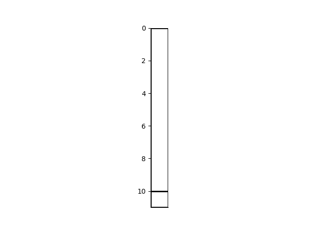
mod.plot_grid(transpose=True, flip=True)

Randomness and Model Perturbations

We can set the priors on the 1D model by assigning minimum and maximum layer depths and a maximum number of layers. These are used to create priors on the number of cells in the model, a new depth interface, new parameter values and the vertical gradient of those parameters. The halfSpaceValue is used as a reference value for the parameter prior.

from numpy.random import Generator
from numpy.random import PCG64DXSM
generator = PCG64DXSM(seed=0)
prng = Generator(generator)

# Set the priors
mod.set_priors(value_mean=0.01,
              min_edge=1.0,
              max_edge=150.0,
              max_cells=30,
              solve_value=True,
              solve_gradient=True,
              prng=prng)

We can evaluate the prior of the model using depths only

print('Log probability of the Model given its priors: ', mod.probability(False, False))
# Or with priors on its parameters, and parameter gradient with depth.
print('Log probability of the Model given its priors: ', mod.probability(True, True))

Log probability of the Model given its priors:  -3.367295829986474
Log probability of the Model given its priors:  -9.157731937350919

To propose new models, we specify the probabilities of creating, removing, perturbing, and not changing a layer interface

pProposal = Distribution('LogNormal', 0.01, np.log(2.0)**2.0, linearSpace=True, prng=prng)
mod.set_proposals(probabilities=[0.25, 0.25, 0.5, 0.25], proposal=pProposal, prng=prng)

We can then perturb the layers of the model

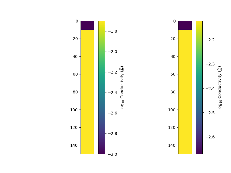
remapped, perturbed = mod.perturb()

fig = plt.figure(figsize=(8, 6))
ax = plt.subplot(121)
mod.pcolor(transpose=True, flip=True, log=10)  # , grid=True)
ax = plt.subplot(122)
perturbed.pcolor(transpose=True, flip=True, log=10)  # , grid=True)

<Axes: >

We can evaluate the prior of the model using depths only

print('Log probability of the Model given its priors: ',perturbed.probability(False, False))
# Or with priors on its parameters, and parameter gradient with depth.
print('Log probability of the Model given its priors: ',perturbed.probability(True, True))

Log probability of the Model given its priors:  -3.367295829986474
Log probability of the Model given its priors:  -8.559817917094882

Perturbing a model multiple times

In the stochasitic inference process, we perturb the model structure, and parameter values, multiple times. Each time the model is perturbed, we can record its state in a posterior distribution.

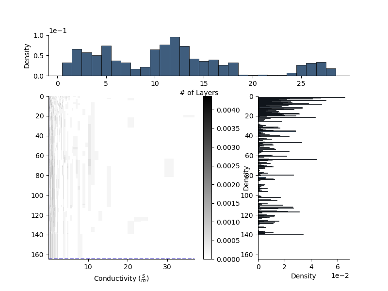
For a 1D model, the parameter posterior is a 2D hitmap with depth in one dimension and the parameter value in the other. We also attach a 1D histogram for the number of layers, and a 1D histogram for the locations of interfaces.

Since we have already set the priors on the Model, we can set the posteriors based on bins from from the priors.

mod.set_posteriors()

mod0 = deepcopy(mod)

Now we randomly perturb the model, and update its posteriors.

mod.update_posteriors()
for i in range(1001):
    remapped, perturbed = mod.perturb()

    # And update the model posteriors
    perturbed.update_posteriors()

    mod = perturbed

We can now plot the posteriors of the model.

Remember in this case, we are simply perturbing the model structure and parameter values The proposal for the parameter values is fixed and centred around a single value. fig = plt.figure(figsize=(8, 6))

# plt.subplot(131)
# mod.nCells.posterior.plot()
# ax = plt.subplot(132)
# mod.values.posterior.pcolor(cmap='gray_r', colorbar=False, flipY=True, logX=10)
# plt.subplot(133, sharey=ax)
# mod.mesh.edges.posterior.plot(transpose=True, flipY=True)

# plt.figure()
# mod.plot_posteriors(**{"cmap": 'gray_r',
#                   "xscale": 'log',
#                   "noColorbar": True,
#                   "flipY": True,
#                   'credible_interval_kwargs':{'axis': 1,
#                                           'reciprocate': True,
#                                           'xscale': 'log'}})
# mod.par.posterior.plotCredibleIntervals(xscale='log', axis=1)


fig = plt.figure(figsize=(8, 6))
# gs = fig.add_gridspec(nrows=1, ncols=1)
mod.plot_posteriors(axes=fig,
                    edges_kwargs = {
                        "transpose":True,
                        "flipY":True
                    },
                    parameter_kwargs = {
                        "cmap": 'gray_r',
                        "xscale": 'log',
                        "colorbar": False,
                        "flipY": True,
                        'credible_interval_kwargs':{
                              'reciprocate':True,
                            #   'axis': 1,
                              'xscale': 'log'
                        }
                    },
                    best = mod)


plt.show()