Note
Go to the end to download the full example code.
ASEG-GDF (Tempest AEM)
This example demonstrates the workflow for creating a GS file from the ASEG file format, as well as how to add multiple associated datasets to the Survey. Specifically, this AEM survey contains the following datasets:
Raw AEM data, from the Tempest system
Inverted resistivity models
An interpolated map of total magnetic intensity
Source Reference: Minsley, B.J., James, S.R., Bedrosian, P.A., Pace, M.D., Hoogenboom, B.E., and Burton, B.L., 2021, Airborne electromagnetic, magnetic, and radiometric survey of the Mississippi Alluvial Plain, November 2019 - March 2020: U.S. Geological Survey data release, https://doi.org/10.5066/P9E44CTQ.
import matplotlib.pyplot as plt
from os.path import join
import gspy
Initialize the Survey
# Path to example files
data_path = "..//data_files//tempest_aseg"

# Survey Metadata file
metadata = join(data_path, "data//Tempest_survey_md.yml")

# Establish survey instance
survey = gspy.Survey.from_dict(metadata)
 1dataset_attrs:
 2    title: Example Tempest Airborne Electromagnetic (AEM) Dataset
 3    institution: USGS Geology, Geophysics, & Geochemistry Science Center
 4    source:  Contractor provided ASEG-GDF2 formatted data
 5    history: This example dataset includes the raw AEM data and gridded magnetic data as provided by the contractor, CGG Canada Services, Ltd, as well as 1-D resistivity models inverted by the USGS using the GALEISBSTDEM time-domain deterministic inversion software (Brodie 2015, Geoscience Australia, Release-20160606).
 6    references: "Minsley, B.J., James, S.R., Bedrosian, P.A., Pace, M.D., Hoogenboom, B.E., and Burton, B.L., 2021, Airborne electromagnetic, magnetic, and radiometric survey of the Mississippi Alluvial Plain, November 2019 - March 2020: U.S. Geological Survey data release, https://doi.org/10.5066/P9E44CTQ."
 7    comment: This dataset is incomplete and has been downsampled for the purposes of this example.
 8    content: Tempest AEM Survey from the Mississippi Alluvial Plain
 9
10spatial_ref:
11    wkid: 5070
12    authority: EPSG
13
14survey_information:
15    contractor_project_number: 603756FWA
16    contractor: CGG Canada Services Ltd.
17    client: U.S. Geological Survey
18    survey_type: electromagneticmagneticradiometric
19    survey_area_name: Mississippi Alluvial Plain (MAP)
20    state: MO,AR,TN,MS,LA,IL,KY
21    country: USA
22    acquisition_start: 20191120
23    acquisition_end: 20200307
24    dataset_created: 20200420
25
26survey_units:
27    time: seconds [s]
28    area: square meters [m^2]
29    current: Amperes [A]
30    frequency: Hertz [Hz]
31    electromagnetic_moment: Ampere square meters [Am^2]
32    magnetometer_b_field: nano Tesla [nT]
33    electromagnetic_b_field: femto tesla [fT]
34
35flightline_information:
36    traverse_line_spacing: 6000
37    traverse_line_direction: various
38    nominal_terrain_clearance: 120
39    final_line_kilometers: 24868
40    TRAVERSE LINE NUMBERS: "[192401 - 265021, 400801 - 401401, 500101, 604501 - 608101, 700201 - 700206, 710101 - 710401]"
41    REPEAT LINE NUMBERS: 9100071 - 9180772
42    PRE ZERO LINE NUMBERS: 90200702 - 90207701
43    POST ZERO LINE NUMBERS: 90500702 - 90507701
44
45survey_equipment:
46    aircraft: Cessna C208B
47    aircraft_registration: VH-FHY
48    magnetometer: Bartington MAG-03MS100 three-axis fluxgate
49    magnetometer_installation: Stinger mounted
50    electromagnetic_system: 30Hz TEMPEST
51    electromagnetic_installation: Transmitter loop mounted on the aircraft, Reciver coils in a towed bird
52    electromagnetic_coil_orientations: X,Z
53    spectrometer_system: Radiation Solutions RS-500
54    spectrometer_installation: Mounted in the aircraft
55    radar_altimeter_system: Collins Alt-50
56    radar_altimeter_sample_rate: 0.1 s
57    laser_altimeter_system: Riegl LD90-3
58    laser_altimeter_sample_rate: 0.1 s
59    navigation_system: Real-time differential GPS
60    navigation_sample_rate: 1.0 s
61    acquisition_system: FASDAS
Create a branch and attach data leaves
Create the first branch (container) called “data”
data_container = survey.gs.add_container('data', **dict(content = "raw data"))
Raw Data
Import raw AEM data from ASEG-GDF2 format.
d_data = join(data_path, 'data//Tempest.dat')
d_supp = join(data_path, 'data//Tempest_data_md.yml')

# Add the raw AEM data to the data branch
rd = data_container.gs.add(key='raw_data',
                           data=d_data,
                           metadata_file=d_supp)
Note for ASEG-GDF2 files, variable metadata is pulled directly from the DFN file associated with the DAT file. Any additional variable metadata, or desired overwrites to the DFN values, can be passed through the YAML.
In this example, multiple systems are defined in the Tempest_data_md.yml metadata file:
  1dataset_attrs:
  2    content: raw AEM data
  3    comment: This dataset includes minimally processed (raw) AEM data
  4    type: data
  5    mode: airborne
  6    method: [magnetic, radiometric, "electromagnetic, time domain"]
  7    instrument: 30Hz Tempest
  8
  9coordinates:
 10    x: Easting_Albers
 11    y: Northing_Albers
 12    z: DTM
 13
 14tempest_system:
 15    type: system
 16    mode: airborne
 17    method: electromagnetic, time domain
 18    instrument: 30Hz Tempest
 19
 20    dimensions:
 21        gate_times:
 22            standard_name: gate_times
 23            long_name: receiver gate times
 24            units: seconds
 25            missing_value: not_defined
 26            bounds: [[5.430000e-06, 1.628000e-05],
 27                        [2.713000e-05, 3.798000e-05],
 28                        [4.883000e-05, 5.968000e-05],
 29                        [7.053000e-05, 1.030800e-04],
 30                        [1.139400e-04, 1.681900e-04],
 31                        [1.790400e-04, 2.767000e-04],
 32                        [2.875500e-04, 4.503200e-04],
 33                        [4.611700e-04, 7.107400e-04],
 34                        [7.215900e-04, 1.101380e-03],
 35                        [1.112230e-03, 1.709030e-03],
 36                        [1.719880e-03, 2.663920e-03],
 37                        [2.674770e-03, 4.161360e-03],
 38                        [4.172210e-03, 6.505170e-03],
 39                        [6.516030e-03, 1.008600e-02],
 40                        [1.009686e-02, 1.666171e-02]]
 41            centers: [1.085000e-05, 3.255000e-05, 5.426000e-05, 8.681000e-05,
 42                1.410600e-04, 2.278700e-04, 3.689300e-04, 5.859500e-04,
 43                9.114800e-04, 1.410630e-03, 2.191900e-03, 3.418070e-03,
 44                5.338690e-03, 8.301020e-03, 1.337928e-02]
 45
 46    variables:
 47
 48        data_normalized: True
 49        output_data_type: B
 50        reference_frame: right-handed positive up
 51        output_sample_frequency: 5
 52        digitization_frequency: 92160
 53
 54        transmitter:
 55            label: Z
 56            area: 155
 57            waveform_type: square
 58            waveform_time:
 59                values: [-1.66666667e-02, -1.66612413e-02, -5.4255e-06,  0.0, 5.4255e-06,  1.66612413e-02,  1.66666667e-02]
 60                long_name: not_defined
 61                missing_value: not_defined
 62                units: s
 63            waveform_current:
 64                values: [0.0,  1.0,  1.0,  0.0, -1.0, -1.0,  0.0]
 65                dimensions: 'waveform_time'
 66            scale_factor: 0.5
 67            peak_current: 560
 68            peak_moment: 86800
 69            base_frequency: 30
 70            orientation: Z
 71            number_of_turns: 1
 72            on_time: 0.00833
 73            off_time: 0.00833
 74
 75        receiver:
 76            label: [z, x]
 77            orientation: [z, x]
 78
 79        couplet:
 80            transmitters: [z, z]
 81            receivers: [z, x]
 82            txrx_dx: [-120, -120]
 83            txrx_dy: [0, 0]
 84            txrx_dz: [-52, -52]
 85
 86variables:
 87    Easting_Albers:
 88        long_name: Easting_Albers:PROJECTION=WGS84/Albers
 89    Northing_Albers:
 90        long_name: Northing_Albers:PROJECTION=WGS84/Albers
 91    DTM:
 92        positive: up
 93        datum: NAD88
 94    EMX_NonHPRG:
 95        system_couplet: z_x
 96        dimensions: [index, gate_times]
 97    EMX_HPRG:
 98        system_couplet: z_x
 99        dimensions: [index, gate_times]
100    EMZ_NonHPRG:
101        system_couplet: z_z
102        dimensions: [index, gate_times]
103    EMZ_HPRG:
104        system_couplet: z_z
105        dimensions: [index, gate_times]
Create a 2nd branch and attach model data leaves
model_container = survey.gs.add_container('models', **dict(content = "inverted 1-D electrical resistivity models"))

# Define Path to inverted AEM models and corresponding metadata file
m_data = join(data_path, 'model//Tempest_model.dat')
m_supp = join(data_path, 'model//Tempest_model_md.yml')

# Add models to the model container, note this example contains a "parameters" group that
# is added as a leaflet below the model group.
mod = model_container.gs.add(key='inverted_models',
                             data=m_data,
                             metadata_file=m_supp,
                             system=rd.tempest_system,
                             derived_from=rd)
  1dataset_attrs:
  2    content: inverted resistivity models
  3    comment: This dataset includes inverted resistivity models derived from processed AEM data produced by USGS
  4    type: model
  5    method: electromagnetic, time domain
  6    instrument: 30Hz Tempest
  7    mode: airborne
  8    property: electrical conductivity
  9
 10coordinates:
 11    x: easting
 12    y: northing
 13    z: elevation
 14
 15dimensions:
 16    layer_depth:
 17        standard_name: layer_depth
 18        long_name: inverted model layer depth
 19        units: m
 20        missing_value: not_defined
 21        bounds: [[  0.0  ,   3.0  ],
 22                    [  3.0  ,   6.3 ],
 23                    [  6.3 ,   9.93],
 24                    [  9.93,  13.92],
 25                    [ 13.92,  18.31],
 26                    [ 18.31,  23.14],
 27                    [ 23.14,  28.45],
 28                    [ 28.45,  34.3 ],
 29                    [ 34.3 ,  40.73],
 30                    [ 40.73,  47.8 ],
 31                    [ 47.8 ,  55.58],
 32                    [ 55.58,  64.14],
 33                    [ 64.14,  73.56],
 34                    [ 73.56,  83.92],
 35                    [ 83.92,  95.31],
 36                    [ 95.31, 107.84],
 37                    [107.84, 121.62],
 38                    [121.62, 136.78],
 39                    [136.78, 153.46],
 40                    [153.46, 171.8 ],
 41                    [171.8 , 191.98],
 42                    [191.98, 214.18],
 43                    [214.18, 238.6 ],
 44                    [238.6 , 265.46],
 45                    [265.46, 295.01],
 46                    [295.01, 327.51],
 47                    [327.51, 363.26],
 48                    [363.26, 402.59],
 49                    [402.59, 445.85],
 50                    [445.85, 489.11]]
 51        centers: [  1.5  ,   4.65 ,   8.115,  11.925,  16.115,  20.725,  25.795,
 52                    31.375,  37.515,  44.265,  51.69 ,  59.86 ,  68.85 ,  78.74 ,
 53                    89.615, 101.575, 114.73 , 129.2  , 145.12 , 162.63 , 181.89 ,
 54                    203.08 , 226.39 , 252.03 , 280.235, 311.26 , 345.385, 382.925,
 55                    424.22 , 467.48 ]
 56
 57    gate_times:
 58        standard_name: gate_times
 59        long_name: receiver gate times
 60        units: seconds
 61        missing_value: not_defined
 62        bounds: [[5.430000e-06, 1.628000e-05],
 63                    [2.713000e-05, 3.798000e-05],
 64                    [4.883000e-05, 5.968000e-05],
 65                    [7.053000e-05, 1.030800e-04],
 66                    [1.139400e-04, 1.681900e-04],
 67                    [1.790400e-04, 2.767000e-04],
 68                    [2.875500e-04, 4.503200e-04],
 69                    [4.611700e-04, 7.107400e-04],
 70                    [7.215900e-04, 1.101380e-03],
 71                    [1.112230e-03, 1.709030e-03],
 72                    [1.719880e-03, 2.663920e-03],
 73                    [2.674770e-03, 4.161360e-03],
 74                    [4.172210e-03, 6.505170e-03],
 75                    [6.516030e-03, 1.008600e-02],
 76                    [1.009686e-02, 1.666171e-02]]
 77        centers: [1.085000e-05, 3.255000e-05, 5.426000e-05, 8.681000e-05,
 78            1.410600e-04, 2.278700e-04, 3.689300e-04, 5.859500e-04,
 79            9.114800e-04, 1.410630e-03, 2.191900e-03, 3.418070e-03,
 80            5.338690e-03, 8.301020e-03, 1.337928e-02]
 81
 82variables:
 83    elevation:
 84        positive: up
 85        datum: NAD88
 86
 87    conductivity:
 88        dimensions: [index, layer_depth]
 89
 90    thickness:
 91        dimensions: [index, layer_depth]
 92
 93    observed_EMSystem_1_XS:
 94        system_couplet: z_x
 95        dimensions: [index, gate_times]
 96
 97    observed_EMSystem_1_ZS:
 98        system_couplet: z_z
 99        dimensions: [index, gate_times]
100
101    noise_EMSystem_1_XS:
102        system_couplet: z_x
103        dimensions: [index, gate_times]
104
105    noise_EMSystem_1_ZS:
106        system_couplet: z_z
107        dimensions: [index, gate_times]
108
109    predicted_EMSystem_1_XS:
110        system_couplet: z_x
111        dimensions: [index, gate_times]
112
113    predicted_EMSystem_1_ZS:
114        system_couplet: z_z
115        dimensions: [index, gate_times]
116
117inversion_parameters:
118    dataset_attrs:
119        type: parameters
120        method: electromagnetic, time domain
121        instrument: 30Hz Tempest
122        mode: airborne
123        property: electrical conductivity
124
125    variables:
126        software: GALEISBSTDEM 1-D time-domain deterministic inversion software
127        software_reference: "Brodie, R. C., 2015, GALEISBSTDEM: A deterministic algorithm for 1D sample by sample inversion of time-domain AEM data – theoretical details, accessed May 1, 2020, at https://github.com/GeoscienceAustralia/ga-aem/blob/master/docs/GALEISBSTDEM%20Inversion%20Algorithm%20Theoretical%20Details%20.pdf."
128        description: Inversions were done using a multilayered smooth model formulation in which 30 layer thicknesses were fixed and layer conductivities were solved for. Horizontal (X) and vertical (Z) components of the data were inverted separately. A vertical conductivity smoothing constraint, alpha_s = 1000, was applied. The inversion reference model used a half-space conductivity of 0.04 Siemens per meter (S/m) with a standard deviation of 1 S/m. The relative importance of the reference conductivity model, alpha_c, was set to 1.0. The horizontal and vertical separation between transmitter and receiver was given a lateral and vertical standard deviation constraint of 0.5 meters (m) in the reference model. The receiver pitch was also included with a 0.5 m standard deviation. These steps were repeated using the same inversion parameters but for reference models of higher (0.2 S/m) and lower (0.008 S/m) conductivity representing lower (5 Ohm-m) and higher (125) resistivity, respectively. A number of inversions were conducted with various homogenous prior model values, and constraints on resistivity. The final model parameters described above were selected because they best represent the physical understanding of the system and minimized data misfit. Final inverted resistivity values for each layer, layer thicknesses, and the uncertainty associated with these values can be found in the model dataset.
129        doi_calculation: The depth of investigation (DOI) for each model location was calculated using the difference between the low and high reference conductivity model results. Using the approach from Oldenburg and Li (1999), models from the low and high reference inversions were divided and rescaled producing a metric of their similarity. Models were similar where constrained by the data (shallow depths) and diverge back to their distinct reference model values when no longer constrained by the data. Therefore, the DOI was calculated as the threshold below which models were no longer informed by the data.
130        phid_cut: Individual models with a data misfit, "PhiD", less than or equal to 1.5 were accepted for final outputs and products. A new channel, "ACCEPT_FLAG" was added to the data file representing this misfit cutoff, with 0 = rejected models and 1 = accepted models.
Create a 3rd branch for the magnetic intensity map
# Create a new branch for the contractor-derived total magnetic intensity map
map_container = survey.gs.add_container('derived_maps', **dict(content = "derived maps"))

# Import the magnetic data from TIF-format.
d_supp = join(data_path, 'data//Tempest_raster_md.yml')

# Add the magnetic map to the data
maps = map_container.gs.add(key='maps', metadata_file = d_supp)
Note: raster data files are defined within the metadata file
  1dataset_attrs:
  2    comment: contractor-derived product
  3    content: gridded map of total magnetic intensity
  4    type: data
  5    mode: airborne
  6    method: magnetic
  7    instrument: Scintrex CS-3 cesium vapor magnetometer
  8
  9magnetic_system:
 10    type: system
 11    mode: airborne
 12    method: magnetic
 13    instrument: Scintrex CS-3 c cesium-vapor magnetometer
 14
 15    prefixes: ['base_magnetometer']
 16
 17    dimensions:
 18        base_mag_locations:
 19            standard_name: base_mag_locations
 20            long_name: Base Magnetometer Location Index Numbers
 21            units: not_defined
 22            missing_value: not_defined
 23            length: 6
 24            increment: 1
 25            origin: 1
 26
 27    variables:
 28        transmitter:
 29            label: passive
 30            description: No artificial transmitter was used; the system measures the Earth's natural magnetic field (passive field).
 31
 32        receiver:
 33            label: scalar_magnetometer
 34            sensor_type: cesium_vapor
 35            sensor_model: CS-3
 36            sensor_manufacturer: Scintrex
 37            description: Scalar cesium-vapor magnetometer mounted in the aircraft tail stinger.
 38                Magnetic samples are processed by a FASDAS magnetometer processor
 39                board and synchronized via GPS PPS; a Bartington MAG-03MS100
 40                three-axis fluxgate provides aircraft attitude for compensation.
 41            orientation: tail-stinger mounted
 42            coordinates:
 43                values: "[-10.74, 0.0, -0.55]"
 44                long_name: magnetometer location relative to Tx loop center (X,Y,Z)
 45                units: meters
 46            acquisition_system: FASDAS survey/magnetometer computer; NovAtel OEMV-3 GPS with
 47                OMNISTAR differential corrections; dynamic compensation driven by IMU
 48                and fluxgate attitude inputs. A tail stinger mounted Bartington MAG-03MS100 three-axis fluxgate magnetometer is used to provide information on the attitude of the aircraft. This information is used for compensation of the measured magnetic total field.
 49            sample_frequency:
 50                values: 0.2
 51                units: s
 52            sensitivity:
 53                values: 0.001
 54                units: nT
 55            typical_noise:
 56                values: 1.0
 57                units: nT
 58            compensation: fully digital
 59            parallax:
 60                values: 1.8
 61                units: s
 62
 63        base_magnetometer:
 64            label: base_magnetometer
 65            description: Ground magnetic base stations established at low-gradient sites; two CF1 magnetometers operated continuously at 1 s sampling with ~0.01 nT sensitivity. Base data edited to remove spikes/level shifts and used for diurnal correction per base location.
 66            sensor_type: CF1 magnetometer
 67            sample_frequency:
 68                values: 1
 69                units: s
 70            sensitivity:
 71                values: 0.01
 72                units: nT
 73
 74            location_names:
 75                values: ["Greenwood, MS", "Alexandria, LA", "Monroe, LA", "West Memphis, AR", "Sikeston, MO", "Greenwood, MS"]
 76                dimensions: 'base_mag_locations'
 77
 78            flights:
 79                values: ["007-027", "028-036", "038-042", "044-062", "063-074", "075-077"]
 80                dimensions: 'base_mag_locations'
 81
 82            values:
 83                values: [49170.0, 47640.7, 48362.6, 50083.5, 51678.8, 49170.0]
 84                dimensions: 'base_mag_locations'
 85
 86
 87        dynamic_compensation: Compensation calibration flights at high altitude; pitches/rolls/yaws used to derive coefficients that remove aircraft-induced magnetic noise. Reported improvement ratio ~2.91 (std. dev. uncompensated vs. compensated).
 88        diurnal_correction: Diurnal base values applied by location (see base_magnetometer section); base data edited and filtered to remove non-geophysical disturbances.
 89        igrf_model_date: "2019-12-01"
 90        igrf_model_height: "167.9 m"
 91        igrf_removed_model_epoch: "2015.0"
 92        tieline_levelling: RMI levelled to prior RESOLVE data; due to height differences and limited tie lines, manual adjustments and micro-levelling were applied.
 93        deliverables: "Total Magnetic Intensity (TMI), provided with EM & terrain data"
 94
 95        couplet:
 96            transmitters: [passive]
 97            receivers: [scalar_magnetometer]
 98            description: Passive Earth field transmitter paired with single scalar magnetometer receiver mounted in tail stinger.
 99
100coordinates:
101    x: Easting_Albers
102    y: Northing_Albers
103
104dimensions:
105    x: Easting_Albers
106    y: Northing_Albers
107
108variables:
109    magnetic_tmi:
110        dimensions: [x, y]
111        system_couplet: passive_scalar_magnetometer
112        standard_name: total_magnetic_intensity
113        long_name: Total magnetic intensity, diurnally corrected and filtered
114        units: nT
115        missing_value: 1.70141e+38
116        files: [mag.tif]
117
118    Easting_Albers:
119        standard_name: easting_albers
120        long_name: Easting
121        units: meter
122        missing_value: not_defined
123
124    Northing_Albers:
125        standard_name: northing_albers
126        long_name: Northing
127        units: meter
128        missing_value: not_defined
Save NetCDF file
d_out = join(data_path, 'Tempest.nc')
survey.gs.to_netcdf(d_out)
Read back in the NetCDF file
new_survey = gspy.open_datatree(d_out)['survey']
View the Data Tree
print(new_survey)
<xarray.DataTree 'survey'>
Group: /survey
│ Dimensions: ()
│ Coordinates:
│ spatial_ref float64 8B ...
│ Data variables:
│ survey_information float64 8B ...
│ survey_units float64 8B ...
│ flightline_information float64 8B ...
│ survey_equipment float64 8B ...
│ Attributes:
│ type: survey
│ title: Example Tempest Airborne Electromagnetic (AEM) Dataset
│ institution: USGS Geology, Geophysics, & Geochemistry Science Center
│ source: Contractor provided ASEG-GDF2 formatted data
│ history: This example dataset includes the raw AEM data and gridded...
│ references: Minsley, B.J., James, S.R., Bedrosian, P.A., Pace, M.D., H...
│ comment: This dataset is incomplete and has been downsampled for th...
│ content: Tempest AEM Survey from the Mississippi Alluvial Plain /su...
│ gspy_version: 2.2.8
│ conventions: GS-2.0, CF-1.13
├── Group: /survey/data
│ │ Dimensions: ()
│ │ Data variables:
│ │ spatial_ref float64 8B ...
│ │ Attributes:
│ │ content: raw data
│ │ type: container
│ └── Group: /survey/data/raw_data
│ │ Dimensions: (index: 2001, gate_times: 15)
│ │ Coordinates:
│ │ * index (index) float64 16kB 0.0 1.0 2.0 ... 1.999e+03 2e+03
│ │ * gate_times (gate_times) float64 120B 1.085e-05 3.255e-05 ... 0.01338
│ │ spatial_ref float64 8B ...
│ │ x (index) float64 16kB ...
│ │ y (index) float64 16kB ...
│ │ z (index) float64 16kB ...
│ │ Data variables: (12/58)
│ │ line (index) float64 16kB ...
│ │ flight (index) float64 16kB ...
│ │ fiducial (index) float64 16kB ...
│ │ proj_cgg (index) float64 16kB ...
│ │ proj_client (index) float64 16kB ...
│ │ date (index) float64 16kB ...
│ │ ... ...
│ │ z_primaryfield (index) float64 16kB ...
│ │ z_vlf1 (index) float64 16kB ...
│ │ z_vlf2 (index) float64 16kB ...
│ │ z_vlf3 (index) float64 16kB ...
│ │ z_vlf4 (index) float64 16kB ...
│ │ z_geofact (index) float64 16kB ...
│ │ Attributes:
│ │ content: raw AEM data
│ │ comment: This dataset includes minimally processed (raw) AEM data
│ │ type: data
│ │ mode: airborne
│ │ method: ['magnetic', 'radiometric', 'electromagnetic, time domain']
│ │ instrument: 30Hz Tempest
│ │ structure: tabular
│ └── Group: /survey/data/raw_data/tempest_system
│ Dimensions: (gate_times: 15, nv: 2, n_transmitter: 1,
│ waveform_time: 7, n_receiver: 2,
│ n_couplet: 2, dim_0: 1)
│ Coordinates:
│ * nv (nv) float64 16B 0.0 1.0
│ * n_transmitter (n_transmitter) float64 8B 0.0
│ * waveform_time (waveform_time) float64 56B -0.01667 ... 0....
│ * n_receiver (n_receiver) float64 16B 0.0 1.0
│ * n_couplet (n_couplet) float64 16B 0.0 1.0
│ Dimensions without coordinates: dim_0
│ Data variables: (12/26)
│ gate_times_bnds (gate_times, nv) float64 240B ...
│ transmitter_label (n_transmitter) <U1 4B ...
│ transmitter_area (n_transmitter) int64 8B ...
│ transmitter_waveform_type (n_transmitter) <U6 24B ...
│ transmitter_waveform_current (waveform_time) float64 56B ...
│ transmitter_scale_factor (n_transmitter) float64 8B ...
│ ... ...
│ couplet_txrx_dz (n_couplet) int64 16B ...
│ data_normalized (dim_0) bool 1B ...
│ output_data_type <U1 4B ...
│ reference_frame <U24 96B ...
│ output_sample_frequency (dim_0) int64 8B ...
│ digitization_frequency (dim_0) int64 8B ...
│ Attributes:
│ type: system
│ mode: airborne
│ method: electromagnetic, time domain
│ instrument: 30Hz Tempest
│ name: tempest_system
├── Group: /survey/models
│ │ Dimensions: ()
│ │ Data variables:
│ │ spatial_ref float64 8B ...
│ │ Attributes:
│ │ content: inverted 1-D electrical resistivity models
│ │ type: container
│ └── Group: /survey/models/inverted_models
│ │ Dimensions: (layer_depth: 30, nv: 2, gate_times: 15,
│ │ index: 2001)
│ │ Coordinates:
│ │ * layer_depth (layer_depth) float64 240B 1.5 4.65 ... 424.2 467.5
│ │ * nv (nv) float64 16B 0.0 1.0
│ │ * gate_times (gate_times) float64 120B 1.085e-05 ... 0.01338
│ │ * index (index) float64 16kB 0.0 1.0 ... 1.999e+03 2e+03
│ │ spatial_ref float64 8B ...
│ │ x (index) float64 16kB ...
│ │ y (index) float64 16kB ...
│ │ z (index) float64 16kB ...
│ │ Data variables: (12/46)
│ │ layer_depth_bnds (layer_depth, nv) float64 480B ...
│ │ gate_times_bnds (gate_times, nv) float64 240B ...
│ │ uniqueid (index) float64 16kB ...
│ │ survey (index) float64 16kB ...
│ │ date (index) float64 16kB ...
│ │ flight (index) float64 16kB ...
│ │ ... ...
│ │ phic (index) float64 16kB ...
│ │ phit (index) float64 16kB ...
│ │ phig (index) float64 16kB ...
│ │ phis (index) float64 16kB ...
│ │ lambda (index) float64 16kB ...
│ │ iterations (index) float64 16kB ...
│ │ Attributes:
│ │ content: inverted resistivity models
│ │ comment: This dataset includes inverted resistivity models derived fr...
│ │ type: model
│ │ method: electromagnetic, time domain
│ │ instrument: 30Hz Tempest
│ │ mode: airborne
│ │ property: electrical conductivity
│ │ structure: tabular
│ ├── Group: /survey/models/inverted_models/tempest_system
│ │ Dimensions: (gate_times: 15, nv: 2, n_transmitter: 1,
│ │ waveform_time: 7, n_receiver: 2,
│ │ n_couplet: 2, dim_0: 1)
│ │ Coordinates:
│ │ * n_transmitter (n_transmitter) float64 8B 0.0
│ │ * waveform_time (waveform_time) float64 56B -0.01667 ... 0....
│ │ * n_receiver (n_receiver) float64 16B 0.0 1.0
│ │ * n_couplet (n_couplet) float64 16B 0.0 1.0
│ │ Dimensions without coordinates: dim_0
│ │ Data variables: (12/26)
│ │ gate_times_bnds (gate_times, nv) float64 240B ...
│ │ transmitter_label (n_transmitter) <U1 4B ...
│ │ transmitter_area (n_transmitter) int64 8B ...
│ │ transmitter_waveform_type (n_transmitter) <U6 24B ...
│ │ transmitter_waveform_current (waveform_time) float64 56B ...
│ │ transmitter_scale_factor (n_transmitter) float64 8B ...
│ │ ... ...
│ │ couplet_txrx_dz (n_couplet) int64 16B ...
│ │ data_normalized (dim_0) bool 1B ...
│ │ output_data_type <U1 4B ...
│ │ reference_frame <U24 96B ...
│ │ output_sample_frequency (dim_0) int64 8B ...
│ │ digitization_frequency (dim_0) int64 8B ...
│ │ Attributes:
│ │ type: system
│ │ mode: airborne
│ │ method: electromagnetic, time domain
│ │ instrument: 30Hz Tempest
│ │ name: tempest_system
│ └── Group: /survey/models/inverted_models/inversion_parameters
│ Dimensions: ()
│ Data variables:
│ software <U61 244B ...
│ software_reference <U298 1kB ...
│ description <U1402 6kB ...
│ doi_calculation <U592 2kB ...
│ phid_cut <U256 1kB ...
│ Attributes:
│ type: parameters
│ method: electromagnetic, time domain
│ instrument: 30Hz Tempest
│ mode: airborne
│ property: electrical conductivity
│ name: inversion_parameters
└── Group: /survey/derived_maps
│ Dimensions: ()
│ Data variables:
│ spatial_ref float64 8B ...
│ Attributes:
│ content: derived maps
│ type: container
└── Group: /survey/derived_maps/maps
│ Dimensions: (x: 599, nv: 2, y: 1212)
│ Coordinates:
│ * x (x) float64 5kB 2.928e+05 2.934e+05 ... 6.51e+05 6.516e+05
│ * nv (nv) float64 16B 0.0 1.0
│ * y (y) float64 10kB 1.607e+06 1.606e+06 ... 8.808e+05 8.802e+05
│ spatial_ref float64 8B ...
│ Data variables:
│ x_bnds (x, nv) float64 10kB ...
│ y_bnds (y, nv) float64 19kB ...
│ magnetic_tmi (y, x) float64 6MB ...
│ Attributes:
│ comment: contractor-derived product
│ content: gridded map of total magnetic intensity
│ type: data
│ mode: airborne
│ method: magnetic
│ instrument: Scintrex CS-3 cesium vapor magnetometer
│ structure: raster
└── Group: /survey/derived_maps/maps/magnetic_system
Dimensions: (base_mag_locations: 6, nv: 2,
n_transmitter: 1, n_receiver: 1,
n_couplet: 1, n_base_magnetometer: 1)
Coordinates:
* base_mag_locations (base_mag_locations) float64 48B 1.0 ...
* n_transmitter (n_transmitter) float64 8B 0.0
* n_receiver (n_receiver) float64 8B 0.0
* n_couplet (n_couplet) float64 8B 0.0
* n_base_magnetometer (n_base_magnetometer) float64 8B 0.0
Data variables: (12/35)
base_mag_locations_bnds (base_mag_locations, nv) float64 96B ...
transmitter_label (n_transmitter) <U7 28B ...
transmitter_description (n_transmitter) <U107 428B ...
receiver_label (n_receiver) <U19 76B ...
receiver_sensor_type (n_receiver) <U12 48B ...
receiver_sensor_model (n_receiver) <U4 16B ...
... ...
diurnal_correction <U142 568B ...
igrf_model_date <U10 40B ...
igrf_model_height <U7 28B ...
igrf_removed_model_epoch <U6 24B ...
tieline_levelling <U137 548B ...
deliverables <U63 252B ...
Attributes:
type: system
mode: airborne
method: magnetic
instrument: Scintrex CS-3 c cesium-vapor magnetometer
name: magnetic_system
Once the survey is read in, we can access variables like a standard xarray dataset.
Option A:
print(new_survey['derived_maps/maps'].magnetic_tmi)
<xarray.DataArray 'magnetic_tmi' (y: 1212, x: 599)> Size: 6MB
[725988 values with dtype=float64]
Coordinates:
  * y            (y) float64 10kB 1.607e+06 1.606e+06 ... 8.808e+05 8.802e+05
  * x            (x) float64 5kB 2.928e+05 2.934e+05 ... 6.51e+05 6.516e+05
    spatial_ref  float64 8B ...
Attributes:
    system_couplet:  passive_scalar_magnetometer
    standard_name:   total_magnetic_intensity
    long_name:       Total magnetic intensity, diurnally corrected and filtered
    units:           nT
    valid_range:     [-17504.6640625   11490.32324219]
    grid_mapping:    spatial_ref
Option B:
print(new_survey['derived_maps/maps']['magnetic_tmi'])
<xarray.DataArray 'magnetic_tmi' (y: 1212, x: 599)> Size: 6MB
[725988 values with dtype=float64]
Coordinates:
  * y            (y) float64 10kB 1.607e+06 1.606e+06 ... 8.808e+05 8.802e+05
  * x            (x) float64 5kB 2.928e+05 2.934e+05 ... 6.51e+05 6.516e+05
    spatial_ref  float64 8B ...
Attributes:
    system_couplet:  passive_scalar_magnetometer
    standard_name:   total_magnetic_intensity
    long_name:       Total magnetic intensity, diurnally corrected and filtered
    units:           nT
    valid_range:     [-17504.6640625   11490.32324219]
    grid_mapping:    spatial_ref
Option C:
print(new_survey['derived_maps']['maps']['magnetic_tmi'])
<xarray.DataArray 'magnetic_tmi' (y: 1212, x: 599)> Size: 6MB
[725988 values with dtype=float64]
Coordinates:
  * y            (y) float64 10kB 1.607e+06 1.606e+06 ... 8.808e+05 8.802e+05
  * x            (x) float64 5kB 2.928e+05 2.934e+05 ... 6.51e+05 6.516e+05
    spatial_ref  float64 8B ...
Attributes:
    system_couplet:  passive_scalar_magnetometer
    standard_name:   total_magnetic_intensity
    long_name:       Total magnetic intensity, diurnally corrected and filtered
    units:           nT
    valid_range:     [-17504.6640625   11490.32324219]
    grid_mapping:    spatial_ref
Plotting Examples
demonstrating different ways to access and plot variables
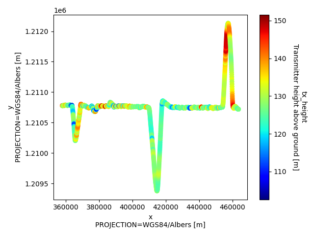
# Make a scatter plot of a specific tabular variable, using GSPy's plotter
plt.figure()
new_survey['data']['raw_data'].gs.scatter(x='x', hue='tx_height', cmap='jet')
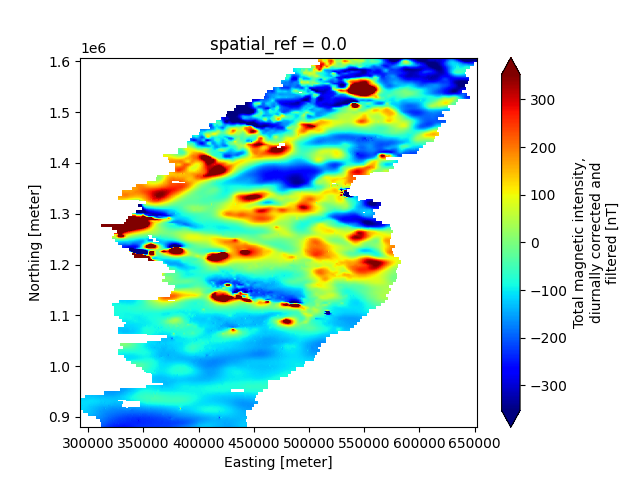
Make a 2-D map plot of a specific raster variable, using Xarrays’s plotter
plt.figure()
new_survey['derived_maps/maps']['magnetic_tmi'].plot(cmap='jet', robust=True)
plt.show()
Total running time of the script: (0 minutes 1.462 seconds)