Note
Go to the end to download the full example code.
GeoTIFFs (2D & 3D)
In this example, we demonstrate the workflow for creating a GS file from the GeoTIFF (.tif/.tiff) file format. This includes adding individual TIF files as single 2-D variables, as well as how to create a 3-D variable by stacking multiple TIF files along a specified dimension.
The GS standard requires a single set of x, y, z, t coordinate variables per data leaf group. Therefore, this example also shows how tifs with differing x-y grids need to be added to separate groups, and all variables in a group should have matching coordinates:
- Raster Dataset #1
2-D magnetic grid, original x-y discretization (600 m cell size)
- Raster Dataset #2
2-D magnetic grid, aligned to match the x-y dimensions of the resistivity layers (1000 m cell size)
3-D resistivity grid
Lastly, GSPy provides a “to_tif()” method to export raster data as GeoTIFF. This example demonstrates how to use this method for both 2D and 3D variables.
Source References:
Minsley, B.J., James, S.R., Bedrosian, P.A., Pace, M.D., Hoogenboom, B.E., and Burton, B.L., 2021, Airborne electromagnetic, magnetic, and radiometric survey of the Mississippi Alluvial Plain, November 2019 - March 2020: U.S. Geological Survey data release, https://doi.org/10.5066/P9E44CTQ.
James, S.R., and Minsley, B.J., 2021, Combined results and derivative products of hydrogeologic structure and properties from airborne electromagnetic surveys in the Mississippi Alluvial Plain: U.S. Geological Survey data release, https://doi.org/10.5066/P9382RCI.
import matplotlib.pyplot as plt
from os.path import join
import gspy
from gspy import Survey
Initialize the Survey
# Path to example files
data_path = "..//data_files//tempest_aseg"

# Survey metadata file
metadata = join(data_path, "data//Tempest_survey_md.yml")

# Establish the Survey
survey = Survey.from_dict(metadata)
 1dataset_attrs:
 2    title: Example Tempest Airborne Electromagnetic (AEM) Dataset
 3    institution: USGS Geology, Geophysics, & Geochemistry Science Center
 4    source:  Contractor provided ASEG-GDF2 formatted data
 5    history: This example dataset includes the raw AEM data and gridded magnetic data as provided by the contractor, CGG Canada Services, Ltd, as well as 1-D resistivity models inverted by the USGS using the GALEISBSTDEM time-domain deterministic inversion software (Brodie 2015, Geoscience Australia, Release-20160606).
 6    references: "Minsley, B.J., James, S.R., Bedrosian, P.A., Pace, M.D., Hoogenboom, B.E., and Burton, B.L., 2021, Airborne electromagnetic, magnetic, and radiometric survey of the Mississippi Alluvial Plain, November 2019 - March 2020: U.S. Geological Survey data release, https://doi.org/10.5066/P9E44CTQ."
 7    comment: This dataset is incomplete and has been downsampled for the purposes of this example.
 8    content: Tempest AEM Survey from the Mississippi Alluvial Plain
 9
10spatial_ref:
11    wkid: 5070
12    authority: EPSG
13
14survey_information:
15    contractor_project_number: 603756FWA
16    contractor: CGG Canada Services Ltd.
17    client: U.S. Geological Survey
18    survey_type: electromagneticmagneticradiometric
19    survey_area_name: Mississippi Alluvial Plain (MAP)
20    state: MO,AR,TN,MS,LA,IL,KY
21    country: USA
22    acquisition_start: 20191120
23    acquisition_end: 20200307
24    dataset_created: 20200420
25
26survey_units:
27    time: seconds [s]
28    area: square meters [m^2]
29    current: Amperes [A]
30    frequency: Hertz [Hz]
31    electromagnetic_moment: Ampere square meters [Am^2]
32    magnetometer_b_field: nano Tesla [nT]
33    electromagnetic_b_field: femto tesla [fT]
34
35flightline_information:
36    traverse_line_spacing: 6000
37    traverse_line_direction: various
38    nominal_terrain_clearance: 120
39    final_line_kilometers: 24868
40    TRAVERSE LINE NUMBERS: "[192401 - 265021, 400801 - 401401, 500101, 604501 - 608101, 700201 - 700206, 710101 - 710401]"
41    REPEAT LINE NUMBERS: 9100071 - 9180772
42    PRE ZERO LINE NUMBERS: 90200702 - 90207701
43    POST ZERO LINE NUMBERS: 90500702 - 90507701
44
45survey_equipment:
46    aircraft: Cessna C208B
47    aircraft_registration: VH-FHY
48    magnetometer: Bartington MAG-03MS100 three-axis fluxgate
49    magnetometer_installation: Stinger mounted
50    electromagnetic_system: 30Hz TEMPEST
51    electromagnetic_installation: Transmitter loop mounted on the aircraft, Reciver coils in a towed bird
52    electromagnetic_coil_orientations: X,Z
53    spectrometer_system: Radiation Solutions RS-500
54    spectrometer_installation: Mounted in the aircraft
55    radar_altimeter_system: Collins Alt-50
56    radar_altimeter_sample_rate: 0.1 s
57    laser_altimeter_system: Riegl LD90-3
58    laser_altimeter_sample_rate: 0.1 s
59    navigation_system: Real-time differential GPS
60    navigation_sample_rate: 1.0 s
61    acquisition_system: FASDAS
Create a branch for all maps
container = survey.gs.add_container('derived_products',
                                    **dict(content = "container of gridded maps of magnetic and electrical resistivity values",
                                           comment = "Magnetic map is contractor-derived, resistivity maps are USGS-derived"))
Attach the 2D Magnetic Raster Dataset (600 m cell size)
Define input metadata file, which contains the TIF filename linked with desired variable name and info.
d_supp1 = join(data_path, 'data//Tempest_raster_md.yml')

# Attach the magnetic map to the container
mm = container.gs.add(key="mag_map", metadata_file=d_supp1)
  1dataset_attrs:
  2    comment: contractor-derived product
  3    content: gridded map of total magnetic intensity
  4    type: data
  5    mode: airborne
  6    method: magnetic
  7    instrument: Scintrex CS-3 cesium vapor magnetometer
  8
  9magnetic_system:
 10    type: system
 11    mode: airborne
 12    method: magnetic
 13    instrument: Scintrex CS-3 c cesium-vapor magnetometer
 14
 15    prefixes: ['base_magnetometer']
 16
 17    dimensions:
 18        base_mag_locations:
 19            standard_name: base_mag_locations
 20            long_name: Base Magnetometer Location Index Numbers
 21            units: not_defined
 22            missing_value: not_defined
 23            length: 6
 24            increment: 1
 25            origin: 1
 26
 27    variables:
 28        transmitter:
 29            label: passive
 30            description: No artificial transmitter was used; the system measures the Earth's natural magnetic field (passive field).
 31
 32        receiver:
 33            label: scalar_magnetometer
 34            sensor_type: cesium_vapor
 35            sensor_model: CS-3
 36            sensor_manufacturer: Scintrex
 37            description: Scalar cesium-vapor magnetometer mounted in the aircraft tail stinger.
 38                Magnetic samples are processed by a FASDAS magnetometer processor
 39                board and synchronized via GPS PPS; a Bartington MAG-03MS100
 40                three-axis fluxgate provides aircraft attitude for compensation.
 41            orientation: tail-stinger mounted
 42            coordinates:
 43                values: "[-10.74, 0.0, -0.55]"
 44                long_name: magnetometer location relative to Tx loop center (X,Y,Z)
 45                units: meters
 46            acquisition_system: FASDAS survey/magnetometer computer; NovAtel OEMV-3 GPS with
 47                OMNISTAR differential corrections; dynamic compensation driven by IMU
 48                and fluxgate attitude inputs. A tail stinger mounted Bartington MAG-03MS100 three-axis fluxgate magnetometer is used to provide information on the attitude of the aircraft. This information is used for compensation of the measured magnetic total field.
 49            sample_frequency:
 50                values: 0.2
 51                units: s
 52            sensitivity:
 53                values: 0.001
 54                units: nT
 55            typical_noise:
 56                values: 1.0
 57                units: nT
 58            compensation: fully digital
 59            parallax:
 60                values: 1.8
 61                units: s
 62
 63        base_magnetometer:
 64            label: base_magnetometer
 65            description: Ground magnetic base stations established at low-gradient sites; two CF1 magnetometers operated continuously at 1 s sampling with ~0.01 nT sensitivity. Base data edited to remove spikes/level shifts and used for diurnal correction per base location.
 66            sensor_type: CF1 magnetometer
 67            sample_frequency:
 68                values: 1
 69                units: s
 70            sensitivity:
 71                values: 0.01
 72                units: nT
 73
 74            location_names:
 75                values: ["Greenwood, MS", "Alexandria, LA", "Monroe, LA", "West Memphis, AR", "Sikeston, MO", "Greenwood, MS"]
 76                dimensions: 'base_mag_locations'
 77
 78            flights:
 79                values: ["007-027", "028-036", "038-042", "044-062", "063-074", "075-077"]
 80                dimensions: 'base_mag_locations'
 81
 82            values:
 83                values: [49170.0, 47640.7, 48362.6, 50083.5, 51678.8, 49170.0]
 84                dimensions: 'base_mag_locations'
 85
 86
 87        dynamic_compensation: Compensation calibration flights at high altitude; pitches/rolls/yaws used to derive coefficients that remove aircraft-induced magnetic noise. Reported improvement ratio ~2.91 (std. dev. uncompensated vs. compensated).
 88        diurnal_correction: Diurnal base values applied by location (see base_magnetometer section); base data edited and filtered to remove non-geophysical disturbances.
 89        igrf_model_date: "2019-12-01"
 90        igrf_model_height: "167.9 m"
 91        igrf_removed_model_epoch: "2015.0"
 92        tieline_levelling: RMI levelled to prior RESOLVE data; due to height differences and limited tie lines, manual adjustments and micro-levelling were applied.
 93        deliverables: "Total Magnetic Intensity (TMI), provided with EM & terrain data"
 94
 95        couplet:
 96            transmitters: [passive]
 97            receivers: [scalar_magnetometer]
 98            description: Passive Earth field transmitter paired with single scalar magnetometer receiver mounted in tail stinger.
 99
100coordinates:
101    x: Easting_Albers
102    y: Northing_Albers
103
104dimensions:
105    x: Easting_Albers
106    y: Northing_Albers
107
108variables:
109    magnetic_tmi:
110        dimensions: [x, y]
111        system_couplet: passive_scalar_magnetometer
112        standard_name: total_magnetic_intensity
113        long_name: Total magnetic intensity, diurnally corrected and filtered
114        units: nT
115        missing_value: 1.70141e+38
116        files: [mag.tif]
117
118    Easting_Albers:
119        standard_name: easting_albers
120        long_name: Easting
121        units: meter
122        missing_value: not_defined
123
124    Northing_Albers:
125        standard_name: northing_albers
126        long_name: Northing
127        units: meter
128        missing_value: not_defined
Attach 3D Resistivity Grids + Aligned 2D Magnetic Raster (1000 m cell size)
Import both 3-D resistivity and 2-D magnetic data, aligned onto a common 1000 m x 1000 m grid
d_supp2 = join(data_path, 'data//Tempest_rasters_md.yml')

# Attach rasters to the container
rm = container.gs.add(key="all_maps", metadata_file=d_supp2)
 1dataset_attrs:
 2    comment: resistivity models are USGS-derived, the total magnetic intensity map is contractor-derived
 3    content: interpolated resistivity models (3-D depth grid) and total magnetic intensity map (2-D)
 4    type: data, models
 5    method: ["electromagnetic, time domain","magnetic"]
 6    instrument: 30Hz Tempest
 7    mode: airborne
 8    property: electrical resistivity, total magnetic intensity
 9
10coordinates:
11    x: Easting_Albers
12    y: Northing_Albers
13    z: depth
14
15dimensions:
16    x: Easting_Albers
17    y: Northing_Albers
18
19    depth:
20        comment: depth is defined here inside our yaml file in order to stack the resistivity tifs along a third dimension. This depth information is not contained in any of the individual tifs.
21        standard_name: depth
22        long_name: Depth below earth's surface DTM
23        units: m
24        missing_value: not_defined
25        length: 5
26        increment: 5.0
27        origin: 0.0
28        positive: down
29        datum: ground surface
30
31variables:
32    Easting_Albers:
33        standard_name: easting_albers
34        long_name: Easting
35        units: meter
36        missing_value: not_defined
37
38    Northing_Albers:
39        standard_name: northing_albers
40        long_name: Northing
41        units: meter
42        missing_value: not_defined
43
44    resistivity:
45        dimensions: [x, y, z]
46        standard_name: log10_resistivity
47        long_name: Electrical Resistivity on Logarithmic Scale
48        units: log10_ohm_m
49        missing_value: -9999.99
50        files: [resistivity_0_5m.tif,
51                resistivity_5_10m.tif,
52                resistivity_10_15m.tif,
53                resistivity_15_20m.tif,
54                resistivity_20_25m.tif]
55
56    magnetic_tmi:
57        dimensions: [x, y]
58        standard_name: total_magnetic_intensity
59        long_name: Total magnetic intensity, diurnally corrected and filtered
60        units: nT
61        missing_value: -999999
62        files: [mag_aligned.tif]
Note: the stack dimension is defined as “depth” but for the resistivity variable the dimensions are listed as [x, y, z] … this is because under coordinates we are linking the z coordinate dimension to the incoming depth dimension. Therefore the name “depth” ends up not getting used because that dimension becomes “z” instead.
Inspect the data tree
print(survey)
<xarray.DataTree 'survey'>
Group: /survey
│   Dimensions:                 ()
│   Coordinates:
│       spatial_ref             float64 8B 0.0
│   Data variables:
│       survey_information      float64 8B nan
│       survey_units            float64 8B nan
│       flightline_information  float64 8B nan
│       survey_equipment        float64 8B nan
│   Attributes:
│       type:         survey
│       title:        Example Tempest Airborne Electromagnetic (AEM) Dataset
│       institution:  USGS Geology, Geophysics, & Geochemistry Science Center
│       source:       Contractor provided ASEG-GDF2 formatted data
│       history:      This example dataset includes the raw AEM data and gridded ...
│       references:   Minsley, B.J., James, S.R., Bedrosian, P.A., Pace, M.D., Ho...
│       comment:      This dataset is incomplete and has been downsampled for the...
│       content:      Tempest AEM Survey from the Mississippi Alluvial Plain
└── Group: /survey/derived_products
    │   Dimensions:      ()
    │   Data variables:
    │       spatial_ref  float64 8B 0.0
    │   Attributes:
    │       content:  container of gridded maps of magnetic and electrical resistivit...
    │       comment:  Magnetic map is contractor-derived, resistivity maps are USGS-d...
    │       type:     container
    ├── Group: /survey/derived_products/mag_map
    │   │   Dimensions:       (x: 599, nv: 2, y: 1212)
    │   │   Coordinates:
    │   │     * x             (x) float64 5kB 2.928e+05 2.934e+05 ... 6.51e+05 6.516e+05
    │   │     * nv            (nv) int64 16B 0 1
    │   │     * y             (y) float64 10kB 1.607e+06 1.606e+06 ... 8.808e+05 8.802e+05
    │   │       spatial_ref   float64 8B 0.0
    │   │   Data variables:
    │   │       x_bnds        (x, nv) float64 10kB 2.925e+05 2.931e+05 ... 6.519e+05
    │   │       y_bnds        (y, nv) float64 19kB 1.607e+06 1.606e+06 ... 8.799e+05
    │   │       magnetic_tmi  (y, x) float64 6MB nan nan nan nan nan ... nan nan nan nan nan
    │   │   Attributes:
    │   │       comment:     contractor-derived product
    │   │       content:     gridded map of total magnetic intensity
    │   │       type:        data
    │   │       mode:        airborne
    │   │       method:      magnetic
    │   │       instrument:  Scintrex CS-3 cesium vapor magnetometer
    │   │       structure:   raster
    │   └── Group: /survey/derived_products/mag_map/magnetic_system
    │           Dimensions:                             (base_mag_locations: 6, nv: 2,
    │                                                    n_transmitter: 1, n_receiver: 1,
    │                                                    n_couplet: 1, n_base_magnetometer: 1)
    │           Coordinates:
    │             * base_mag_locations                  (base_mag_locations) int64 48B 1 2 ... 6
    │             * n_transmitter                       (n_transmitter) int64 8B 0
    │             * n_receiver                          (n_receiver) int64 8B 0
    │             * n_couplet                           (n_couplet) int64 8B 0
    │             * n_base_magnetometer                 (n_base_magnetometer) int64 8B 0
    │           Data variables: (12/35)
    │               base_mag_locations_bnds             (base_mag_locations, nv) float64 96B ...
    │               transmitter_label                   (n_transmitter) <U7 28B 'passive'
    │               transmitter_description             (n_transmitter) <U107 428B "No artifi...
    │               receiver_label                      (n_receiver) <U19 76B 'scalar_magneto...
    │               receiver_sensor_type                (n_receiver) <U12 48B 'cesium_vapor'
    │               receiver_sensor_model               (n_receiver) <U4 16B 'CS-3'
    │               ...                                  ...
    │               diurnal_correction                  <U142 568B 'Diurnal base values appli...
    │               igrf_model_date                     <U10 40B '2019-12-01'
    │               igrf_model_height                   <U7 28B '167.9 m'
    │               igrf_removed_model_epoch            <U6 24B '2015.0'
    │               tieline_levelling                   <U137 548B 'RMI levelled to prior RES...
    │               deliverables                        <U63 252B 'Total Magnetic Intensity (...
    │           Attributes:
    │               type:        system
    │               mode:        airborne
    │               method:      magnetic
    │               instrument:  Scintrex CS-3 c cesium-vapor magnetometer
    │               name:        magnetic_system
    └── Group: /survey/derived_products/all_maps
            Dimensions:       (z: 5, nv: 2, x: 363, y: 770)
            Coordinates:
              * z             (z) float64 40B 0.0 5.0 10.0 15.0 20.0
              * nv            (nv) int64 16B 0 1
              * x             (x) float64 3kB 2.915e+05 2.925e+05 ... 6.525e+05 6.535e+05
              * y             (y) float64 6kB 1.648e+06 1.647e+06 ... 8.798e+05 8.788e+05
                spatial_ref   float64 8B 0.0
            Data variables:
                z_bnds        (z, nv) float64 80B -2.5 2.5 2.5 7.5 ... 12.5 17.5 17.5 22.5
                x_bnds        (x, nv) float64 6kB 2.91e+05 2.92e+05 ... 6.53e+05 6.54e+05
                y_bnds        (y, nv) float64 12kB 1.648e+06 1.647e+06 ... 8.783e+05
                resistivity   (z, y, x) float64 11MB nan nan nan nan nan ... nan nan nan nan
                magnetic_tmi  (y, x) float32 1MB nan nan nan nan nan ... nan nan nan nan nan
            Attributes:
                comment:     resistivity models are USGS-derived, the total magnetic inte...
                content:     interpolated resistivity models (3-D depth grid) and total m...
                type:        data, models
                method:      ['electromagnetic, time domain', 'magnetic']
                instrument:  30Hz Tempest
                mode:        airborne
                property:    electrical resistivity, total magnetic intensity
                structure:   raster
Save to NetCDF file
d_out = join(data_path, 'tifs.nc')
survey.gs.to_netcdf(d_out)
Option 1:
Pass a variable name to export just that variable
survey['derived_products']["all_maps"].gs.to_tif('magnetic_tmi')
magnetic_tmi.tif
Option 2:
Export all the variables by NOT passing any variable names, but need to specify a slice dimension for the 3D resistivity variable. Can optionally pass a directory path to export tiffs to.
survey['derived_products']["all_maps"].gs.to_tif(slice_dim='z', out_dir=data_path)
../data_files/tempest_aseg/resistivity_0.0.tif
../data_files/tempest_aseg/resistivity_5.0.tif
../data_files/tempest_aseg/resistivity_10.0.tif
../data_files/tempest_aseg/resistivity_15.0.tif
../data_files/tempest_aseg/resistivity_20.0.tif
../data_files/tempest_aseg/magnetic_tmi.tif
Reading back in the GS NetCDF file
new_survey = gspy.open_datatree(d_out)['survey']
Plotting
Make a map-view plot of a specific data variable, using Xarray’s plotter In this case, we slice the 3-D resistivity variable along the depth dimension
r_plot = new_survey['derived_products']["all_maps"]['resistivity'].plot(col='z', vmax=3, cmap='jet', robust=True)

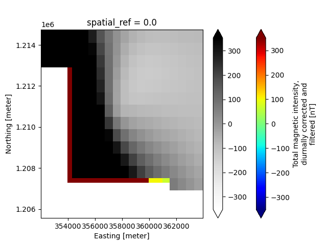
Make a map-view plot comparing the different x-y discretization of the two magnetic variables, using Xarray’s plotter
plt.figure()
ax=plt.gca()
plot1 = new_survey['derived_products']["all_maps"]['magnetic_tmi'].plot(ax=ax, cmap='jet', vmin=0, vmax=1000, robust=True)
plot2 = new_survey['derived_products']["mag_map"]['magnetic_tmi'].plot(ax=ax, cmap='Greys', cbar_kwargs={'label': ''}, robust=True)
plt.ylim([1.20556e6, 1.21476e6])
plt.xlim([3.5201e5, 3.6396e5])
plt.show()
Total running time of the script: (0 minutes 0.764 seconds)