Indexing points to a network

An index ties a point (a streamgage, a sample site, an intake) to a network. index_points_to_lines() finds the flowline nearest each point and returns a position on it: the flowline id and an id_measure along it. Where the network carries an aggregate_id such as a reachcode or mainstem, the index also carries the aggregate_id and an aggregate_id_measure along the whole aggregate flowpath. Both measures are “interpolative” (a percent of the length) and run from 0 at the outlet (downstream end) to 100 at the inlet (upstream end). In contrast, add_hydro_location_distance() records “absolute” measures: a distance in kilometers upstream or downstream of a reference location such as a confluence.

hydroloom indexing functions fall in two groups. The first finds and works with indexes to flowlines and waterbodies:

index_points_to_lines() finds flowlines near each point and returns a position on each.
index_points_to_waterbodies() finds the waterbody each point is in or near and, with flowlines supplied, the flowline at the waterbody’s outlet.
disambiguate_indexes() picks the best of several candidate flowlines per point using a numeric (such as drainage area) or character (such as name) attribute.
get_hydro_location() returns the point on the flowline that an index refers to.
rescale_measures() converts an aggregate_id_measure (such as a reachcode measure) to an id_measure along one flowline.
get_partial_length() returns the length of a flowline below and above an index.
navigate_connected_paths() returns the network distance between the outlets of pairs of flowlines. With get_partial_length(), it gives the network distance between two indexes.

The second records and places positions along identified mainstems, where the aggregate_id is a mainstem identifier:

add_measures() computes aggregate_id from and to measures for flowlines that lack them.
get_confluences() returns a hydro location for each place one identified mainstem enters another.
add_hydro_location_distance() records a position as a signed distance along its mainstem from the nearest hydro location, such as a confluence.
index_hydro_location_distance() places such a distance back on a network as a flowline id and id_measure.
get_subpath() returns the flowline pieces between two positions on one mainstem.

This article covers the first group. The distances from confluences along mainstems article covers the second.

Background

The nearest flowline to a point is not always the “right” one hydrologically. For example, a point near a confluence is near two rivers but can only measure one of them, and a point along a lake shore may be near a flowline that represents flow through the lake. This article works through those cases with the streamgages of an NHDPlusV2 sample dataset from hydrogeofetch: indexing to vertices and at higher precision, resolving ambiguity among nearby flowlines, locating an index on its flowline, indexing to waterbodies, and measuring network distance between two indexes. This article is website-only and does not run on CRAN.

Flowlines

The sample covers part of the Yahara River basin above Lake Kegonsa. The gage layer covers more than the flowlines do, so the comparisons below keep the gages whose flowline (FLComID) is in the sample.

library(hydroloom)
library(dplyr, warn.conflicts = FALSE)

source(system.file("extdata/sample_data.R", package = "hydrogeofetch"))

flowlines <- sf::read_sf(sample_data, "NHDFlowline_Network") |>
  sf::st_zm()

gages <- sf::read_sf(sample_data, "Gage")
gages <- gages[gages$FLComID %in% flowlines$COMID, ]

nrow(flowlines)
#> [1] 267
nrow(gages)
#> [1] 31

search_radius is in the units of the points’ projection, so both layers are projected to Albers (meters) first. The search is a nearest neighbor search against flowline vertices; see the nn2 function from the RANN package for how it works.

flowlines_5070 <- sf::st_transform(flowlines, 5070)
gages_5070 <- sf::st_transform(gages, 5070)

radius <- units::set_units(200, "m")

indexes <- index_points_to_lines(flowlines_5070, gages_5070,
  search_radius = radius)

head(indexes)
#>   point_id    COMID id_measure      REACHCODE REACHCODE_measure     offset
#> 1        1 13293744 48.4383419 07090002007743           48.4383 163.809682
#> 2        2 13294276  9.7109783 07090002008387            9.7110  66.124835
#> 3        3 13294360  1.8673877 07090002008367            1.8674   4.204757
#> 4        4 13294264 55.1518809 07090002007650           55.1519   2.034469
#> 5        5 13293750 42.0270100 07090002007373           42.0270  14.460185
#> 6        6 13294312  0.9796439 07090002008383            0.9796   4.991078

The output column names follow the input: COMID and REACHCODE stay as they were, and the reachcode measure comes back as REACHCODE_measure. point_id is the row of the point in gages.

The gage layer records the flowline and reachcode measure that NHDPlusV2 assigned each gage, so the index can be checked against it.

compare <- function(indexes, gages) {
  i <- left_join(data.frame(point_id = seq_len(nrow(gages))),
    indexes[!duplicated(indexes$point_id), ], by = "point_id")

  same_reach <- !is.na(i$REACHCODE) & i$REACHCODE == gages$REACHCODE

  list(
    same_comid = sum(i$COMID == gages$FLComID, na.rm = TRUE),
    of = nrow(gages),
    measure_difference = round(quantile(
      i$REACHCODE_measure[same_reach] - gages$Measure[same_reach],
      probs = c(0, 0.1, 0.25, 0.5, 0.75, 0.9, 1)), digits = 2))
}

compare(indexes, gages)
#> $same_comid
#> [1] 26
#> 
#> $of
#> [1] 31
#> 
#> $measure_difference
#>    0%   10%   25%   50%   75%   90%  100% 
#> -5.54 -1.02 -0.48  0.06  1.02  6.91 19.59

Of the 31 gages, 26 land on the same flowline, and the reachcode measures of those on the same reachcode differ by up to about 20 (percent of the reachcode length).

Higher precision

Snapping to vertices limits a measure to the positions of the flowline vertices. precision densifies the flowlines near each point to the given spacing in meters (with sf::st_segmentize()) before the search.

indexes <- index_points_to_lines(flowlines_5070, gages_5070,
  search_radius = radius, precision = 10)

compare(indexes, gages)
#> $same_comid
#> [1] 31
#> 
#> $of
#> [1] 31
#> 
#> $measure_difference
#>    0%   10%   25%   50%   75%   90%  100% 
#> -0.45 -0.22 -0.08  0.02  0.11  0.22  0.88

All 31 gages now land on the gage layer’s flowline, and the measure differences fall within 1. The flowline match improves along with the measure: with vertices alone, the nearest vertex can belong to a neighboring flowline, especially where two flowlines share an endpoint.

The gage geometry in the NHDPlusV2 gage layer has already been placed on the flowlines, so this comparison shows that the index recovers NHDPlusV2’s own address for each gage. It says nothing about how far a gage’s reported location is from the network. The next section uses the reported locations.

Resolving ambiguity

The gage layer carries each gage’s reported longitude and latitude (LonSite, LatSite). These sit off the network by up to a few hundred meters, and many of them are within reach of more than one flowline. max_matches returns up to that many candidate flowlines per point, nearest first.

sites <- sf::st_drop_geometry(gages) |>
  filter(!is.na(LonSite)) |>
  sf::st_as_sf(coords = c("LonSite", "LatSite"), crs = 4326)

sites_5070 <- sf::st_transform(sites, 5070)

candidates <- index_points_to_lines(flowlines_5070, sites_5070,
  search_radius = radius, precision = 10, max_matches = 10)

n_candidates <- table(candidates$point_id)
sum(n_candidates > 1)
#> [1] 12

compare(candidates, sites)
#> $same_comid
#> [1] 22
#> 
#> $of
#> [1] 30
#> 
#> $measure_difference
#>    0%   10%   25%   50%   75%   90%  100% 
#> -9.26 -1.18 -0.45  0.04  0.31  1.09  1.27

Taking the nearest candidate puts 22 of the 30 reported sites on the gage layer’s flowline. Twelve sites have more than one candidate.

disambiguate_indexes() picks among the candidates for each point by comparing an attribute of the flowline with an attribute of the point. Numeric attributes pick the smallest difference. Character attributes pick the highest string similarity (utils::adist(), ignoring case). The names of the two data frames are not used; the first column of each joins to the index and the second holds the attribute.

Drainage area is the usual numeric choice. The gage layer uses -999999 for a missing drainage area, which has to be set to NA first; a point with no drainage area drops out of the result.

gage_area <- sites$DASqKm
gage_area[gage_area < 0] <- NA

by_area <- disambiguate_indexes(candidates,
  sf::st_drop_geometry(flowlines[, c("COMID", "TotDASqKM")]),
  data.frame(point_id = seq_len(nrow(sites)), area = gage_area))

compare(by_area, sites)
#> $same_comid
#> [1] 15
#> 
#> $of
#> [1] 30
#> 
#> $measure_difference
#>    0%   10%   25%   50%   75%   90%  100% 
#> -1.37 -1.25 -0.51 -0.22  0.08  0.80 10.93

by_name <- disambiguate_indexes(candidates,
  sf::st_drop_geometry(flowlines[, c("COMID", "GNIS_NAME")]),
  data.frame(point_id = seq_len(nrow(sites)), name = sites$STATION_NM))

compare(by_name, sites)
#> $same_comid
#> [1] 19
#> 
#> $of
#> [1] 30
#> 
#> $measure_difference
#>    0%   10%   25%   50%   75%   90%  100% 
#> -9.26 -1.22 -0.44  0.03  0.33  1.12  1.27

Both do worse against the gage layer than the nearest candidate: 15 of 30 by drainage area and 19 by name. The table shows where they differ.

multi <- as.integer(names(n_candidates[n_candidates > 1]))
fl_area <- function(id) round(flowlines$TotDASqKM[match(id, flowlines$COMID)], 1)

nearest <- candidates[!duplicated(candidates$point_id), ]

data.frame(
  station = substr(sites$STATION_NM[multi], 1, 32),
  gage_area = round(gage_area[multi], 1),
  gage_layer = fl_area(sites$FLComID[multi]),
  nearest = fl_area(nearest$COMID[match(multi, nearest$point_id)]),
  by_area = fl_area(by_area$COMID[match(multi, by_area$point_id)]))
#>                             station gage_area gage_layer nearest by_area
#> 1    TOKEN CREEK AT TOKEN CREEK, WI      62.9       35.7    35.7    42.6
#> 2    LAKE WAUBESA AT MC FARLAND, WI     846.9      841.8   841.8   847.9
#> 3       LAKE MENDOTA AT MADISON, WI     603.5      603.7   610.4   603.7
#> 4  LAKE KEGONSA AT BARBER DRIVE NEA     999.7      893.5     8.9    26.8
#> 5  PHEASANT BRANCH AT CENTURY AVE A      53.9       49.5    49.5    50.3
#> 6  PHEASANT BRANCH AT MOUTH AT MIDD      63.5        8.0    58.4    58.4
#> 7    YAHARA RIVER AT MC FARLAND, WI     846.9      841.8   841.8   847.9
#> 8  YAHARA RIVER AT WESTPORT ROAD NE     305.6      295.7   294.0   295.7
#> 9  LAKE WINGRA OUTLET AT MADISON, W      15.5       13.5    13.5    13.8
#> 10      YAHARA RIVER AT WINDSOR, WI     190.6       63.0    63.0   191.0
#> 11       LAKE WINGRA AT MADISON, WI      15.5       13.5    13.5    13.8
#> 12 YAHARA RIVER AT STATE HIGHWAY 11     295.3      294.0   294.0   295.7

The drainage areas are each flowline’s total drainage area at its outlet. A gage partway along a flowline drains less than that, and the gage’s own drainage area seldom agrees exactly with the network’s. On the same river, the flowline just upstream or downstream of the gage often comes closer in drainage area than the flowline the gage is on (Lake Waubesa and Yahara River at McFarland both pick the flowline with 847.9 km² over the one with 841.8 km²). Drainage area separates a large river from a small tributary well but separates neighboring flowlines on one river poorly. Name has the same trouble on one river — it cannot separate flowlines that share a name — and where a flowline has no name, there is nothing to compare.

The Yahara River at Windsor shows the case drainage area handles well.

windsor <- which(sites$SOURCE_FEA == "05427718")

windsor_candidates <- candidates[candidates$point_id == windsor, ]

left_join(windsor_candidates,
  sf::st_drop_geometry(flowlines[, c("COMID", "GNIS_NAME", "TotDASqKM", "Divergence")]),
  by = "COMID") |>
  select(COMID, GNIS_NAME, TotDASqKM, Divergence, offset)
#>      COMID    GNIS_NAME TotDASqKM Divergence   offset
#> 1 13293456                62.9766          2 32.91072
#> 2 13293452                62.8155          0 57.87255
#> 3 13293432                62.8308          1 57.87255
#> 4 13293454 Yahara River  191.0277          0 66.89999
#> 5 13293430 Yahara River  127.8684          0 72.70174

by_area[by_area$point_id == windsor, ]
#> # A tibble: 1 × 6
#>   point_id    COMID id_measure REACHCODE      REACHCODE_measure offset
#>      <int>    <int>      <dbl> <chr>                      <dbl>  <dbl>
#> 1       26 13293454       96.9 07090002007638              96.9   66.9

The gage reports 190.6 km². The nearest flowline, about 33 m from the reported site, is an unnamed channel draining 63 km² that is coded as the minor path of a divergence, and it is also the flowline the gage layer assigns. The Yahara River flowline draining 191 km² is about 67 m away, and drainage area (and name) pick it. For a question about what the gage drains, the Yahara River flowline is the fit-for-purpose index even though it is neither the nearest flowline nor the gage layer’s.

windsor_site <- sites_5070[windsor, ]

plot(sf::st_geometry(sf::st_buffer(windsor_site, 300)), border = NA)
plot(sf::st_geometry(flowlines_5070), col = "grey70", add = TRUE)
plot(sf::st_geometry(flowlines_5070[flowlines_5070$COMID %in% windsor_candidates$COMID, ]),
  col = "grey30", lwd = 2, add = TRUE)
plot(sf::st_geometry(flowlines_5070[flowlines_5070$COMID == sites$FLComID[windsor], ]),
  col = "orange", lwd = 3, add = TRUE)
plot(sf::st_geometry(flowlines_5070[flowlines_5070$COMID %in%
  by_area$COMID[by_area$point_id == windsor], ]), col = "blue", lwd = 3, add = TRUE)
plot(sf::st_geometry(windsor_site), pch = 16, add = TRUE)

legend("topleft", bty = "n", cex = 0.8,
  legend = c("candidates", "gage layer flowline", "drainage area pick",
    "reported site"),
  col = c("grey30", "orange", "blue", "black"),
  lwd = c(2, 3, 3, NA), pch = c(NA, NA, NA, 16))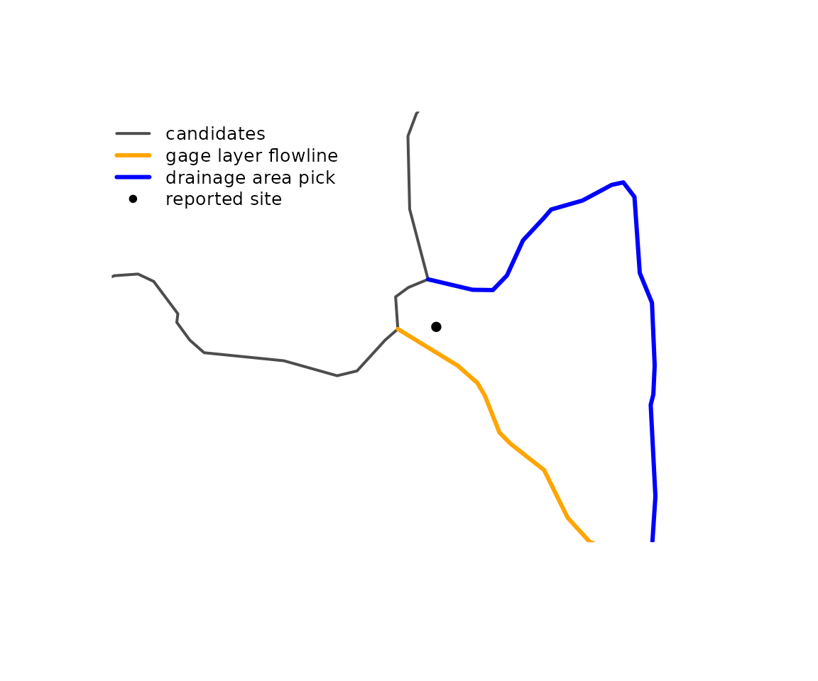

When the right flowline or reachcode is already known, there is nothing to disambiguate. ids (one flowline id per point) and aggregate_ids (one aggregate_id per point) constrain the search instead, so each point can only land on its own flowline or on the flowlines of its own aggregate flowpath. The constraint lets the search radius grow without pulling a point onto a neighbor.

constrained <- index_points_to_lines(flowlines_5070, sites_5070,
  search_radius = units::set_units(500, "m"),
  aggregate_ids = sites$REACHCODE)

compare(constrained, sites)
#> $same_comid
#> [1] 28
#> 
#> $of
#> [1] 30
#> 
#> $measure_difference
#>    0%   10%   25%   50%   75%   90%  100% 
#> -1.59 -1.22 -0.74  0.29  2.26  8.92 30.74

Of the 30 sites, 28 land on the gage layer’s flowline. The other two, on Lake Kegonsa and Lake Monona, are more than 500 m from any flowline on their reachcode and are not indexed; the waterbody section below returns to them.

Locating an index

get_hydro_location() returns the point on the network for each index: the hydro location the index refers to. It interpolates the aggregate_id_measure along the flowline, so the flowlines need the reachcode from and to measures (FromMeas and ToMeas in NHDPlusV2).

located <- get_hydro_location(constrained, flowlines)

plot(sf::st_geometry(flowlines), col = "grey60")
plot(sf::st_geometry(sites)[constrained$point_id], pch = 1, add = TRUE)
plot(located, pch = 16, cex = 0.6, col = "blue", add = TRUE)

legend("topleft", bty = "n", cex = 0.8,
  legend = c("reported site", "hydro location"),
  col = c("black", "blue"), pch = c(1, 16))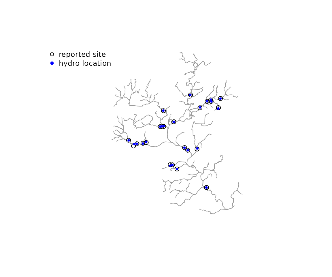

offset in the index is the distance from each point to its hydro location, in the units of the points’ projection (meters here).

round(quantile(constrained$offset))
#>   0%  25%  50%  75% 100% 
#>   11   24   37  103  465

Waterbodies

Seven of the gages are on lakes. For a point on a lake, the nearest flowline is an artificial path through the lake, which stands in for the lake in the network but is not the lake. index_points_to_waterbodies() finds the waterbody each point is in or near and, with flowlines supplied, the flowline at the waterbody’s outlet (the lowest Hydroseq among the flowlines that carry the waterbody’s id).

waterbodies <- sf::read_sf(sample_data, "NHDWaterbody")

lakes <- grepl("LAKE", sites$STATION_NM)

on_lakes <- index_points_to_waterbodies(
  sf::st_transform(waterbodies, 5070),
  sites_5070[lakes, ],
  sf::st_drop_geometry(flowlines),
  search_radius = radius)

cbind(station = substr(sites$STATION_NM[lakes], 1, 32),
  on_lakes,
  gage_layer = sites$FLComID[lakes])
#>                            station near_wb_COMID near_wb_dist in_wb_COMID
#> 1   LAKE WAUBESA AT MC FARLAND, WI     167120949    16.862351          NA
#> 2      LAKE MENDOTA AT MADISON, WI      13293262    22.640184          NA
#> 3 LAKE KEGONSA AT BARBER DRIVE NEA      13296360    50.380329          NA
#> 4       LAKE MONONA AT MADISON, WI      13293316    37.633591    13293316
#> 5 LAKE WINGRA OUTLET AT MADISON, W      13293322     6.737635          NA
#> 6 VILAS BEACH ON LAKE WINGRA AT MA      13293322     3.914543          NA
#> 7       LAKE WINGRA AT MADISON, WI      13293322     6.737635          NA
#>   outlet_fline_COMID gage_layer
#> 1           13294360   13294360
#> 2           13294312   13294312
#> 3           13297172   13302582
#> 4           13294374   13294374
#> 5           13294344   13294344
#> 6           13294344   13294344
#> 7           13294344   13294344

in_wb_COMID is set when a point falls inside a waterbody, and near_wb_COMID names the waterbody with the nearest shoreline within search_radius, at near_wb_dist meters. For six of the seven lake gages, the outlet flowline matches the gage layer’s flowline, including Lake Monona, which the reachcode constraint could not place. The Lake Kegonsa gage gets the outlet of the lake, while the gage layer puts it on another flowline.

Waterbody polygons must be single part. The NHDWaterbody layer stores MULTIPOLYGON geometry with one part each, which is cast to POLYGON; a waterbody with more than one part stops the function with an error.

Network distance between indexes

The network distance between two indexes on the same flow path combines the part of each flowline below its index with the length of the flowlines between them. get_partial_length() returns the lengths below (dn) and above (up) an index on its flowline. navigate_connected_paths() returns the distance from the outlet of one flowline to the outlet of another, which needs the network topology (toid) and length_km.

The Yahara River at Westport Road is above Lake Mendota, and the Yahara River at McFarland is below Lake Monona.

westport <- constrained[constrained$point_id == which(sites$SOURCE_FEA == "05427851"), ]
mcfarland <- constrained[constrained$point_id == which(sites$SOURCE_FEA == "05429500"), ]

westport_partial <- get_partial_length(westport, flowlines)
mcfarland_partial <- get_partial_length(mcfarland, flowlines)

network <- add_toids(hy(sf::st_drop_geometry(flowlines)))

between <- navigate_connected_paths(network, c(westport$COMID, mcfarland$COMID))
between[, c("id_1", "id_2", "network_distance_km")]
#>       id_1     id_2 network_distance_km
#> 1 13294290 13293970              22.946

westport_partial$dn + between$network_distance_km - mcfarland_partial$dn
#> [1] 24.57

The path runs from the outlet of the Westport Road flowline down to the outlet of the McFarland flowline. Adding the part of the Westport Road flowline below its index and removing the part of the McFarland flowline below its index leaves the distance between the two gages along the network.

get_subpath() does this cut directly for two positions on one aggregate flowpath and returns the pieces between them. Recording a position as a distance from a confluence, placing it on another network, and cutting subpaths are the subject of the distances from confluences along mainstems article.