
Distances from confluences along mainstems
dblodgett@usgs.gov
Source:vignettes/articles/mainstem_referencing.Rmd
mainstem_referencing.RmdThis article crosswalks a point from one network to another. The
point is indexed to a flowline (an id and a measure along
it), recorded as a signed distance from the nearest confluence, and
placed on the second network. The same point as a measure along the
whole mainstem (an aggregate_id_measure) is then recorded
as a distance from the same confluence on the second network, and the
two positions compared. Last, get_subpath() cuts the
stretch between two positions, once for one flowline of the first
network on the second and once across a confluence, where the stretch
spans two mainstems.
The NHDPlusV2 flowlines and the mainstem URI lookup ship with hydroloom. The 3DHP sample comes from hydrogeofetch. This article is website-only and does not run on CRAN.
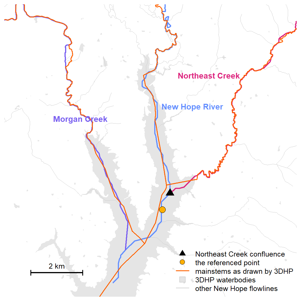
The setting: three identified mainstems in the New Hope sample. The triangle is the confluence used as the hydro location, where Northeast Creek enters the New Hope River, and the dot is the point whose position is recorded as a distance from it. The orange lines are the same three mainstems as 3DHP draws them, over 3DHP waterbodies in grey.
Confluence referenced Hydrologic locations: concepts
A streamgage, a sample site, or an intake is at the outlet of a specific drainage area. That area grows a little at a time with local drainage between confluences and jumps by a whole tributary basin at each one. A position recorded a few hundred meters off along the river, but on the correct side of a confluence, drains nearly the same area as the true position. A position a few meters off but across a confluence does not.
A position indexed to a flowline is that flowline’s id
and a measure along it. A reachcode and measure (an NHD event) is
instead a measure along a reachcode aggregate flowpath;
rescale_measures() converts it to a flowline measure the
same way the HydroAdd3D address is converted below, though that path is
not demonstrated here. The id belongs to a specific
network: the NHDPlusV2 COMID, the NHDPlusHR
nhdplusid, the 3DHP id3dhp. It does not carry
to another network, and the 3DHP id3dhp is not stable
between 3DHP releases.
In contrast, a mainstem URI is durable, and so is a confluence: the place one identified mainstem enters another is present on any network that carries both mainstems. A position recorded as a signed distance along a mainstem from one of its confluences can be placed on any such network, but only approximately, because each network has unique flowline geometry and its own placement of the confluence, so the same distance will land at different points on the ground. What transfers intact is whether the position is upstream or downstream of the confluence.
The two networks
The first network, v2, is a set of flowlines joined to a
lookup of mainstem URIs, with the URI as aggregate_id. A
recipe shipped with hydroloom does the join and casts the flowlines to
LINESTRING so get_subpath() can cut them.
source(system.file("extdata", "new_hope_mainstems.R", package = "hydroloom"))

v2 <- add_toids(hy(new_hope_mainstems))
The second network, net_3dhp, carries mainstem URIs
natively. toid comes from matching
dnhydrosequence to hydrosequence, which also
serves as topo_sort.
source(system.file("extdata", "new_hope_3dhp.R", package = "hydrogeofetch"))

raw_3dhp <- sf::read_sf(sample_new_hope_3dhp)

m <- match(raw_3dhp$dnhydrosequence, raw_3dhp$hydrosequence)
raw_3dhp$toid <- raw_3dhp$id3dhp[m]
raw_3dhp$toid[is.na(raw_3dhp$toid)] <- ""

raw_3dhp <- sf::st_zm(raw_3dhp)
raw_3dhp <- dplyr::transmute(raw_3dhp,
  id = id3dhp, toid = toid, aggregate_id = mainstemid,
  topo_sort = hydrosequence, length_km = lengthkm, divergence = divergence)

net_3dhp <- hy(raw_3dhp)
get_confluences() finds every place one identified
mainstem enters another. Each confluence is a hydro location on the
receiving mainstem, identified by the tributary’s
aggregate_id and placed at the upstream end of the first
receiving flowline below the tributary.
v2conf <- get_confluences(v2)
conf_3dhp <- get_confluences(net_3dhp)

ne_v2 <- v2conf[v2conf$hydro_location_id == ne, ]
ne_3dhp <- conf_3dhp[conf_3dhp$hydro_location_id == ne, ]

ne_v2
#> # A tibble: 1 × 4
#>   aggregate_id                               hydro_location_id     id id_measure
#>   <chr>                                      <chr>              <int>      <dbl>
#> 1 https://geoconnex.us/ref/mainstems/2408056 https://geoconne… 8.89e6        100
ne_3dhp
#> # A tibble: 1 × 4
#>   aggregate_id                               hydro_location_id  id    id_measure
#>   <chr>                                      <chr>              <chr>      <dbl>
#> 1 https://geoconnex.us/ref/mainstems/2408056 https://geoconnex… 30HSV        100
Both networks place the tributary’s confluence (ne) on
the receiving mainstem (nh). The flowline that holds it
differs, as the two id columns show. The confluence is
durable, the flowline is not.
A point on the receiving mainstem
Take a point near the confluence and index it to the receiving
mainstem on the first network, constraining the search with
aggregate_ids and refining the measure with
precision (see resolving
ambiguity in the indexing article).
point <- sf::st_centroid(sf::st_geometry(v2[v2$id == ne_v2$id, ]))
point_sf <- sf::st_sf(geometry = point)

idx <- index_points_to_lines(v2, point_sf, aggregate_ids = nh, precision = 10)
idx
#>   point_id      id id_measure                               aggregate_id
#> 1        1 8894352   49.20647 https://geoconnex.us/ref/mainstems/2408056
#>   aggregate_id_measure  offset
#> 1              49.2065 35.4118
add_hydro_location_distance() records that position as a
signed distance from the nearest hydro location. Passing the one
confluence as the only hydro location measures from it in particular.
The sign is negative because the point sits downstream of the
confluence.
rec <- add_hydro_location_distance(
  data.frame(id = idx$id, id_measure = idx$id_measure), ne_v2, v2)
rec
#>        id id_measure                               aggregate_id
#> 1 8894352   49.20647 https://geoconnex.us/ref/mainstems/2408056
#>                            hydro_location_id distance_km
#> 1 https://geoconnex.us/ref/mainstems/2408627  -0.7542839
Placing the record on the second network
The record is a mainstem, a confluence, and a signed distance.
index_hydro_location_distance() places it on the second
network without reference to the flowline it was recorded on: it finds
the confluence on the second network’s aggregate flowpath axis, adds the
distance, and maps the result to a flowline and measure there.
record <- data.frame(aggregate_id = rec$aggregate_id,
  hydro_location_id = rec$hydro_location_id, distance_km = rec$distance_km)

onto3 <- index_hydro_location_distance(record, ne_3dhp, net_3dhp)
onto3
#>                                 aggregate_id
#> 1 https://geoconnex.us/ref/mainstems/2408056
#>                            hydro_location_id distance_km    id id_measure
#> 1 https://geoconnex.us/ref/mainstems/2408627  -0.7542839 2VMGA   73.83148
#>   past_end_km status
#> 1           0 placed
status is placed: the distance fell within
the mainstem’s flowlines in net_3dhp. past_end
would mean it ran past the downstream or upstream end of those
flowlines, with past_end_km giving how far.
The point and the flowline that holds it on each network, in the same window as the figure at the top of the article:
half <- 5200
ctr <- c(1515500, 1557000)
view <- sf::st_as_sfc(sf::st_bbox(c(xmin = ctr[1] - half, ymin = ctr[2] - half,
  xmax = ctr[1] + half, ymax = ctr[2] + half), crs = sf::st_crs(v2)))

# the three mainstems as the second network draws them
ms_3dhp <- sf::st_transform(
  net_3dhp[!is.na(net_3dhp$aggregate_id) &
    net_3dhp$aggregate_id %in% c(nh, ne, mc), ], sf::st_crs(v2))

# waterbodies of the second network in the window, fetched from the service
wb <- hydrogeofetch::get_3dhp(AOI = sf::st_transform(view, 4326),
  type = "waterbody")
wb <- sf::st_transform(sf::st_zm(wb), sf::st_crs(v2))
nh_v2 <- v2[!is.na(v2$aggregate_id) & v2$aggregate_id == nh, ]
nh_3dhp <- sf::st_transform(
  net_3dhp[!is.na(net_3dhp$aggregate_id) & net_3dhp$aggregate_id == nh, ], sf::st_crs(v2))

v2_line <- nh_v2[nh_v2$id == idx$id, ]
line_3dhp <- nh_3dhp[nh_3dhp$id == onto3$id, ]

plot(view, border = NA, reset = FALSE)
plot(sf::st_geometry(v2), add = TRUE, col = "grey80", lwd = 0.7)
plot(sf::st_geometry(ms_3dhp), add = TRUE, col = "red", lwd = 1)
plot(sf::st_geometry(nh_v2), add = TRUE, col = "lightblue", lwd = 2)
plot(sf::st_geometry(v2_line), add = TRUE, col = "darkblue", lwd = 3)
plot(sf::st_geometry(line_3dhp), add = TRUE, col = "red", lwd = 3)
plot(sf::st_geometry(point_sf), add = TRUE, pch = 16, col = "black")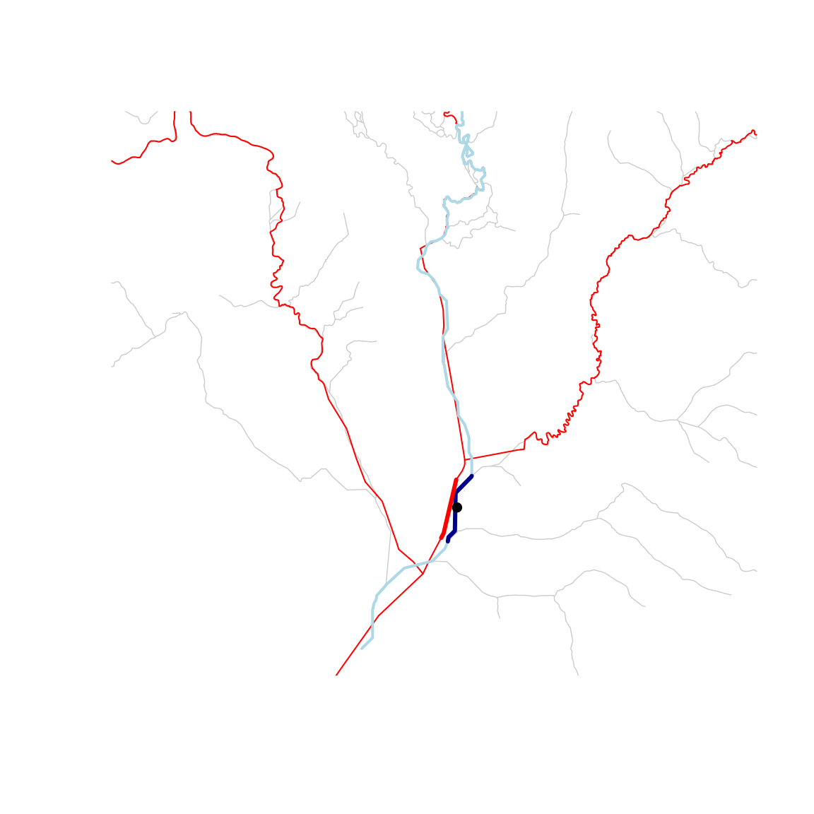
The point (black) sits on the receiving mainstem. The flowline it was indexed to on the first network (dark blue) and the flowline the record was placed on in the second (heavy red, over the second network’s mainstems in thin red) cover the same stretch of river with different lines.
The placed position is approximate. The second network draws the mainstem with its own line and puts the confluence at its own spot on it, so 0.75 km below that spot is not the same point on the ground as 0.75 km below the confluence on the first network. What the record preserves is that the position is downstream of the confluence.
From a mainstem measure
A position can also be given as a measure along a whole mainstem: a
mainstem URI and a measure m, 0 at the mainstem’s
downstream end and 100 at its head. HydroAdd3D (the USGS hydrographic
addressing service for 3DHP) returns locations in this form. The measure
moves whenever the mainstem’s flowlines are edited, extended, or
re-delineated, since a percent of the length changes with the length. A
distance from a confluence holds as long as both mainstems exist.
hydrogeofetch::get_3dhp_index() calls the service; its
example
shows the full response. The address below is written in that shape for
the point used above, with m set to the value hydroloom
gets indexing the same point to the second network.
address <- data.frame(source_id = "1", mainstemid = nh, m = 29.53)m is an aggregate_id_measure in hydroloom
terms. The flowlines of net_3dhp do not carry from and to
measures along the mainstem, so add_measures() computes
them from geometry, projected first so lengths are in meters. It needs
the whole mainstem, which the sample carries.
nh_3dhp_m <- net_3dhp[!is.na(net_3dhp$aggregate_id) & net_3dhp$aggregate_id == nh, ]
nh_3dhp_m <- add_measures(sf::st_transform(nh_3dhp_m, 5070))
The flowline whose measure interval holds m carries the
address, and rescale_measures() converts the mainstem
measure to a measure along that flowline. From there the position is
like any other, and add_hydro_location_distance() records
it as kilometers from the confluence.
fl <- nh_3dhp_m[nh_3dhp_m$aggregate_id_from_measure <= address$m &
  nh_3dhp_m$aggregate_id_to_measure > address$m, ]

pos <- data.frame(id = fl$id,
  id_measure = rescale_measures(address$m, fl$aggregate_id_from_measure,
    fl$aggregate_id_to_measure))

from_address <- add_hydro_location_distance(pos, ne_3dhp, net_3dhp)
from_address
#>      id id_measure                               aggregate_id
#> 1 2VMGA   55.21091 https://geoconnex.us/ref/mainstems/2408056
#>                            hydro_location_id distance_km
#> 1 https://geoconnex.us/ref/mainstems/2408627   -0.977917
The map shows both positions as points on the second network, along
with the input point and its snap onto that network’s line.
st_line_sample() takes a fraction from the first vertex,
which is the upstream end, so the fraction is
1 - id_measure / 100.
on_line <- function(ids, measures) {
  lines <- nh_3dhp_m[match(ids, nh_3dhp_m$id), ]
  sf::st_cast(sf::st_line_sample(lines, sample = 1 - measures / 100), "POINT")
}

p_record <- on_line(onto3$id, onto3$id_measure)
p_address <- on_line(pos$id, pos$id_measure)

point_3d <- sf::st_transform(point_sf, 5070)
snap <- sf::st_nearest_points(point_3d, nh_3dhp_m[nh_3dhp_m$id == pos$id, ])

conf_3d <- sf::st_transform(net_3dhp[net_3dhp$id == ne_3dhp$id, ], 5070)
p_conf <- sf::st_cast(sf::st_line_sample(conf_3d, sample = 0), "POINT")

view <- sf::st_buffer(sf::st_as_sfc(sf::st_bbox(c(p_record, p_address, p_conf))), 300)

all_3d <- sf::st_transform(net_3dhp, 5070)
v2_3d <- sf::st_transform(nh_v2, 5070)

plot(view, border = NA, reset = FALSE)
plot(sf::st_geometry(sf::st_transform(wb, 5070)), add = TRUE, col = "grey90",
  border = NA)
plot(sf::st_geometry(all_3d), add = TRUE, col = "grey70", lwd = 1)
plot(sf::st_geometry(v2_3d), add = TRUE, col = "lightblue", lwd = 3)
plot(sf::st_geometry(nh_3dhp_m), add = TRUE, col = "grey30", lwd = 2)
plot(sf::st_geometry(nh_3dhp_m[nh_3dhp_m$id == pos$id, ]), add = TRUE, col = "red", lwd = 3)
plot(snap, add = TRUE, lty = 2)
plot(sf::st_geometry(point_3d), add = TRUE, pch = 16, col = "black", cex = 1.2)
plot(p_conf, add = TRUE, pch = 17, col = "darkgreen", cex = 1.5)
plot(p_record, add = TRUE, pch = 21, bg = "darkblue", cex = 1.5)
plot(p_address, add = TRUE, pch = 21, bg = "orange", cex = 1.5)

legend("topleft", bty = "n", cex = 0.8,
  legend = c("NHDPlusV2 New Hope River", "3DHP New Hope River",
    "3DHP flowline 2VMGA", "other 3DHP flowlines", "input point",
    "snap onto 3DHP", "Northeast Creek confluence",
    "record transferred from NHDPlusV2", "HydroAdd3D address",
    "3DHP waterbody"),
  col = c("lightblue", "grey30", "red", "grey70", "black", "black",
    "darkgreen", "black", "black", "grey70"),
  lwd = c(3, 2, 3, 1, NA, 1, NA, NA, NA, NA),
  lty = c(1, 1, 1, 1, NA, 2, NA, NA, NA, NA),
  pch = c(NA, NA, NA, NA, 16, NA, 17, 21, 21, 22),
  pt.bg = c(NA, NA, NA, NA, NA, NA, NA, "darkblue", "orange", "grey90"),
  pt.cex = c(NA, NA, NA, NA, 1, NA, 1, 1, 1, 1.8))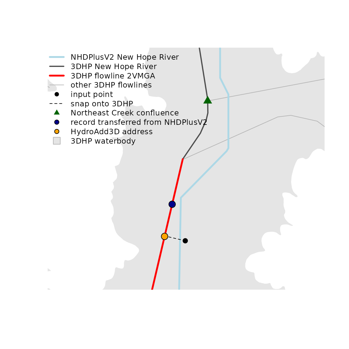
The address (orange) lands on the same flowline as the record transferred from the first network (dark blue), about 0.2 km further downstream of the confluence. The record says 0.75 km below the confluence, measured along the first network’s lines from its placement of the confluence. On the second network that 0.75 km is laid out along different lines from a confluence placed somewhere else. The address instead starts from where the point snaps onto the second network’s line, about 140 m across from it.
The 0.2 km is the approximation in absolute terms: the confluence sits at a different spot on each network, and the kilometers are laid out from wherever each network puts it. The side of the confluence agrees. On both networks the point is downstream of the confluence, so it sees the tributary’s drainage either way. The 0.2 km between the two positions moves the point along the mainstem with no tributary entering between them, which changes its upstream area only by the local drainage along that stretch. Where geometric position has to be exact on the target network, index the original point (or a mainstem measure) on that network rather than transferring the distance.
One flowline’s subpath on the second network
A single flowline of the first network maps to a span of flowlines on
the second. Index both of its ends to the second network with
aggregate_ids, then get_subpath() returns the
ordered pieces between them. An end can sit a few hundred meters from
the second network’s line, so the search radius is raised to 500 m;
aggregate_ids keeps the wider radius from pulling an end
onto a tributary (see resolving
ambiguity).
src <- v2[v2$id == idx$id, ]

e_from <- sf::st_transform(get_node(src, "end"), sf::st_crs(net_3dhp))
e_to <- sf::st_transform(get_node(src, "start"), sf::st_crs(net_3dhp))

rad <- units::set_units(500, "m")
i_from <- index_points_to_lines(net_3dhp, e_from, aggregate_ids = nh, search_radius = rad)
i_to <- index_points_to_lines(net_3dhp, e_to, aggregate_ids = nh, search_radius = rad)

piece <- get_subpath(
  data.frame(id = i_from$id, id_measure = i_from$id_measure),
  data.frame(id = i_to$id, id_measure = i_to$id_measure), net_3dhp)

sf::st_drop_geometry(piece)
#> # A tibble: 2 × 7
#>   line_id segment_order id    id_from_measure id_to_measure length_km reversed
#> *   <int>         <int> <chr>           <dbl>         <dbl>     <dbl> <lgl>
#> 1       1             1 2VMGA               0         100       1.20  FALSE
#> 2       1             2 30HSV               0          50.1     0.220 FALSE
segment_order runs from 1 at the downstream end upward;
id_from_measure and id_to_measure cut the end
pieces; length_km is the piece length. Because
net_3dhp is sf and lwgeom is installed, each
piece also carries its cut geometry.
The source flowline, its two ends snapped onto the second network, and the pieces cut between them:
src_3d <- sf::st_transform(src, 5070)
piece_3d <- sf::st_transform(piece, 5070)
end_from <- sf::st_transform(sf::st_geometry(e_from), 5070)
end_to <- sf::st_transform(sf::st_geometry(e_to), 5070)

snap_from <- sf::st_nearest_points(end_from, nh_3dhp_m[nh_3dhp_m$id == i_from$id, ])
snap_to <- sf::st_nearest_points(end_to, nh_3dhp_m[nh_3dhp_m$id == i_to$id, ])

view <- sf::st_buffer(sf::st_as_sfc(sf::st_bbox(
  c(sf::st_geometry(src_3d), sf::st_geometry(piece_3d)))), 300)

plot(view, border = NA, reset = FALSE)
plot(sf::st_geometry(sf::st_transform(wb, 5070)), add = TRUE, col = "grey90",
  border = NA)
plot(sf::st_geometry(all_3d), add = TRUE, col = "grey70", lwd = 1)
plot(sf::st_geometry(v2_3d), add = TRUE, col = "lightblue", lwd = 3)
plot(sf::st_geometry(src_3d), add = TRUE, col = "darkblue", lwd = 3)
plot(sf::st_geometry(nh_3dhp_m), add = TRUE, col = "grey30", lwd = 2)
plot(sf::st_geometry(piece_3d), add = TRUE, col = "red", lwd = 3)
plot(snap_from, add = TRUE, lty = 2)
plot(snap_to, add = TRUE, lty = 2)
plot(c(end_from, end_to), add = TRUE, pch = 16, col = "black", cex = 1.2)

legend("topleft", bty = "n", cex = 0.8,
  legend = c("NHDPlusV2 New Hope River", "NHDPlusV2 source flowline",
    "3DHP New Hope River", "subpath pieces", "other 3DHP flowlines",
    "source flowline ends", "snap onto 3DHP", "3DHP waterbody"),
  col = c("lightblue", "darkblue", "grey30", "red", "grey70", "black",
    "black", "grey70"),
  lwd = c(3, 3, 2, 3, 1, NA, 1, NA),
  lty = c(1, 1, 1, 1, 1, NA, 2, NA),
  pch = c(NA, NA, NA, NA, NA, 16, NA, 22),
  pt.bg = c(NA, NA, NA, NA, NA, NA, NA, "grey90"),
  pt.cex = c(NA, NA, NA, NA, NA, 1, NA, 1.8))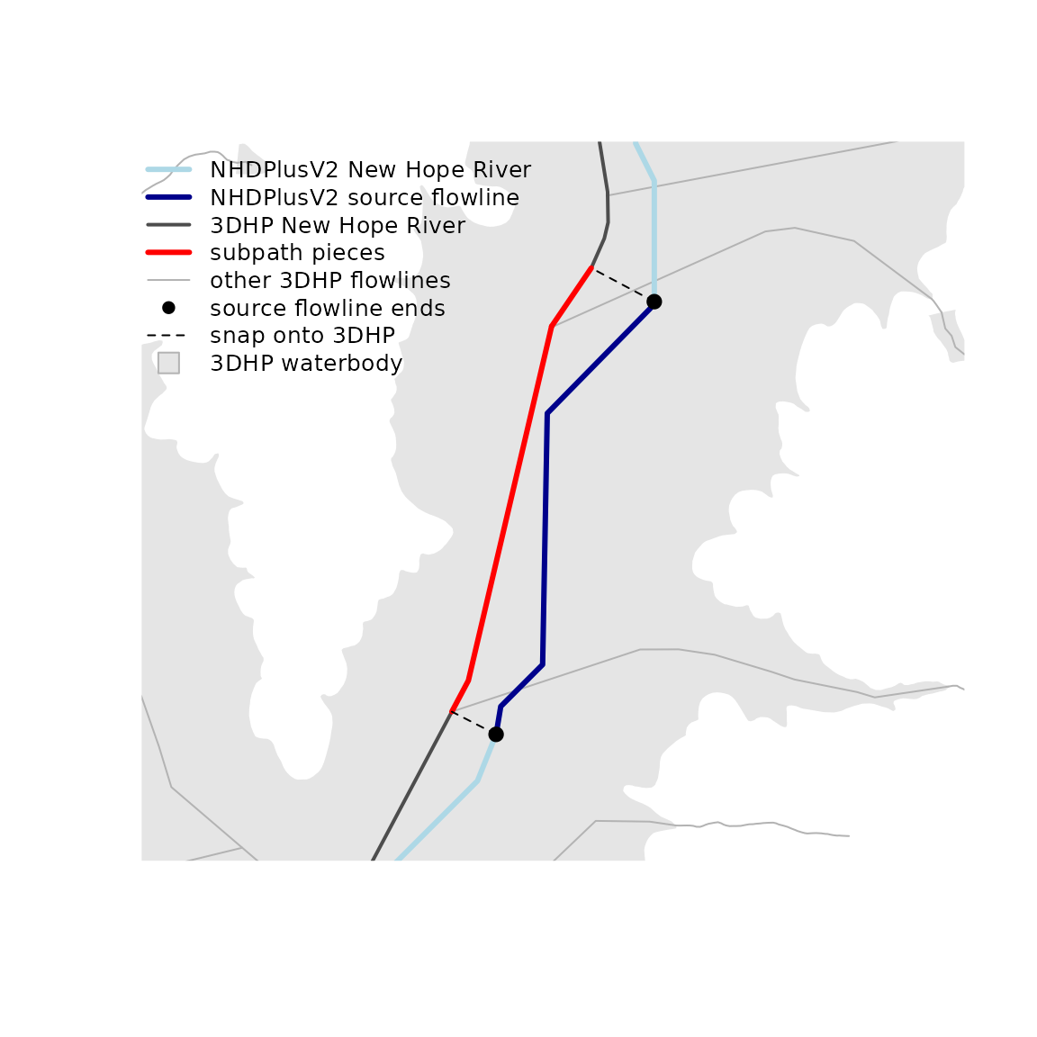
A stretch across a confluence
A stretch from a second tributary (mc) down onto the
receiving mainstem spans two mainstems. get_subpath() takes
two positions on one aggregate flowpath, so the stretch is two calls
split at that tributary’s confluence, which lies on both mainstems.
mc_v2 <- v2conf[v2conf$hydro_location_id == mc, ]

on_mc <- v2[!is.na(v2$aggregate_id) & v2$aggregate_id == mc, ]
on_nh <- v2[!is.na(v2$aggregate_id) & v2$aggregate_id == nh, ]

# Morgan Creek, from an upstream point down to its mouth
up_mc <- data.frame(id = on_mc$id[which.max(on_mc$topo_sort)], id_measure = 100)
mouth_mc <- data.frame(id = on_mc$id[which.min(on_mc$topo_sort)], id_measure = 0)
seg_mc <- get_subpath(up_mc, mouth_mc, v2)

# New Hope River, from the confluence downstream
conf_nh <- data.frame(id = mc_v2$id, id_measure = 100)
down_nh <- data.frame(id = on_nh$id[which.min(on_nh$topo_sort)], id_measure = 0)
seg_nh <- get_subpath(conf_nh, down_nh, v2)

head(sf::st_drop_geometry(seg_mc))
#> # A tibble: 6 × 7
#>   line_id segment_order      id id_from_measure id_to_measure length_km reversed
#>     <int>         <int>   <int>           <dbl>         <dbl>     <dbl> <lgl>
#> 1       1             1 8894358               0           100    1.80   TRUE
#> 2       1             2 8894346               0           100    0.646  TRUE
#> 3       1             3 8897692               0           100    1.69   TRUE
#> 4       1             4 8897678               0           100    1.31   TRUE
#> 5       1             5 8897658               0           100    0.0360 TRUE
#> 6       1             6 8896564               0           100    0.983  TRUE
head(sf::st_drop_geometry(seg_nh))
#> # A tibble: 2 × 7
#>   line_id segment_order      id id_from_measure id_to_measure length_km reversed
#>     <int>         <int>   <int>           <dbl>         <dbl>     <dbl> <lgl>
#> 1       1             1 8897784               0           100    1.39   TRUE
#> 2       1             2 8894360               0           100    0.0450 TRUE
reversed is TRUE because each
from was given upstream of its to; the pieces
still come back downstream to upstream. The two sets meet at the
confluence. To hold the whole stretch as one table, concatenate them in
flow order, the tributary pieces above the receiving mainstem
pieces.