Network Navigation
dblodgett@usgs.gov
Source:vignettes/network_navigation.Rmd
network_navigation.RmdNavigation Modes
Network navigation traverses connections according to a set of rules.
There are four primary modes: upstream or downstream, and along the main
path only or including branches. In hydroloom, these are
upmain, downmain, up, and
down. Additional rules — a maximum distance, for example —
can be applied to any of the four.
hydroloom provides two functions for network
navigation.
-
navigate_network_dfs()requires the “flownetwork” representation of a hydrologic network (seeto_flownetwork()) and returns ids encountered along the requested navigation as a list of contiguous paths. -
navigate_hydro_network()requires the nhdplus representation of a hydrologic network (seevignette("advanced_network")) and returns ids encountered along the requested navigation as a single vector.
Both functions accept the same navigation mode names:
upmain, downmain, up, and
down. navigate_hydro_network() also accepts
the NHDPlus shorthand UM, DM, UT,
and DD.
The two functions use different implementations.
navigate_network_dfs() runs a depth-first search over
upmain and downmain attributes on each
flownetwork connection. navigate_hydro_network() relies on
topo_sort, levelpath, and other nhdplus
attributes.
The rest of this vignette uses the new_hope sample
dataset included with hydroloom. A map and basic summary information are
shown below.
library(hydroloom)
library(sf)

hy_net <- sf::read_sf(system.file("extdata/new_hope.gpkg",
  package = "hydroloom"))

nrow(hy_net)
#> [1] 746

class(hy_net)
#> [1] "sf"         "tbl_df"     "tbl"        "data.frame"

names(hy_net)
#>  [1] "COMID"      "GNIS_ID"    "GNIS_NAME"  "LENGTHKM"   "REACHCODE"
#>  [6] "WBAREACOMI" "FTYPE"      "FCODE"      "StreamLeve" "StreamOrde"
#> [11] "StreamCalc" "FromNode"   "ToNode"     "Hydroseq"   "LevelPathI"
#> [16] "Pathlength" "TerminalPa" "ArbolateSu" "Divergence" "StartFlag"
#> [21] "TerminalFl" "DnLevel"    "UpLevelPat" "UpHydroseq" "DnLevelPat"
#> [26] "DnMinorHyd" "DnDrainCou" "DnHydroseq" "FromMeas"   "ToMeas"
#> [31] "RtnDiv"     "VPUIn"      "VPUOut"     "AreaSqKM"   "TotDASqKM"
#> [36] "geom"

class(hy(hy_net, clean = TRUE))
#> [1] "hy_node"    "hy"         "tbl_df"     "tbl"        "data.frame"

names(hy(hy_net, clean = TRUE))
#>  [1] "id"                        "length_km"
#>  [3] "aggregate_id"              "wbid"
#>  [5] "feature_type"              "feature_type_code"
#>  [7] "stream_level"              "stream_order"
#>  [9] "stream_calculator"         "fromnode"
#> [11] "tonode"                    "topo_sort"
#> [13] "levelpath"                 "pathlength_km"
#> [15] "terminal_topo_sort"        "arbolate_sum"
#> [17] "divergence"                "start_flag"
#> [19] "terminal_flag"             "dn_stream_level"
#> [21] "up_levelpath"              "up_topo_sort"
#> [23] "dn_levelpath"              "dn_minor_topo_sort"
#> [25] "dn_topo_sort"              "aggregate_id_from_measure"
#> [27] "aggregate_id_to_measure"   "da_sqkm"
#> [29] "total_da_sqkm"

# map utilities
map_prep <- \(x, tol = 100) {
  sf::st_geometry(x) |> # no attributes
  sf::st_transform(3857) |> # basemap projection
  sf::st_simplify(dTolerance = tol) # cleaner rendering
}

pc <- list(flowline = list(col = NA)) # to hide flowlines in basemap

oldpar <- par(mar = c(0, 0, 0, 0)) # par is reset in cleanup
nhdplusTools::plot_nhdplus(bbox = sf::st_bbox(hy_net), plot_config = pc)

plot(map_prep(hy_net), col = "blue", add = TRUE)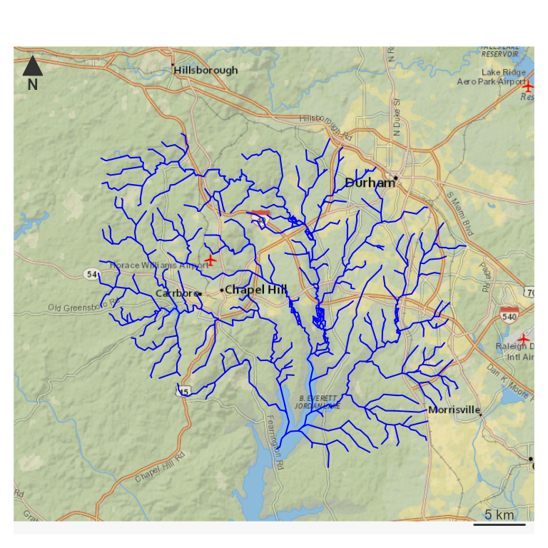
NHDPlus-based network navigation
The nhdplus data model carries network attributes —
levelpath chief among them — that provide a shortcut to
“main” navigations. Flowlines from an upstream headwater down to the
outlet of a given levelpath share the same
levelpath id. Each feature also carries
up_levelpath and dn_levelpath, the
levelpath of the flowline upstream and downstream along the
main path.
levelpath is the key to the algorithm, but
navigate_hydro_network() also draws on
topo_sort, dn_toposort,
dn_minor_hydro, length_km, and
pathlength_km.
When working with data that uses the nhdplus data model,
navigate_hydro_network() runs with no pre-processing.
Below, all four navigation modes are demonstrated using the sample data
as it is provided in NHDPlusV2.
First, we can extract some key features that will help illustrate the network navigation functionality. In line comments illustrate what is being done.
# work in hydroloom attribute names for demo sake
hy_net <- hy(hy_net)
# the smallest topo_sort is the most downstream
outlet <- hy_net[hy_net$topo_sort == min(hy_net$topo_sort), ]
# features with the levelpath of the outlet are the mainpath,
# or mainstem of the network
main_path <- hy_net[hy_net$levelpath == outlet$levelpath, ]
# the largest topo sort along the main path is its headwater flowline
headwater <- main_path[main_path$topo_sort == max(main_path$topo_sort), ]
# basemap
par(mar = c(0, 0, 0, 0))
nhdplusTools::plot_nhdplus(bbox = sf::st_bbox(hy_net), plot_config = pc)
# plot the elements prepped above
plot(map_prep(hy_net), col = "dodgerblue2", add = TRUE, lwd = 0.5)
plot(map_prep(outlet), col = "magenta", add = TRUE, lwd = 4)
plot(map_prep(headwater), col = "magenta", add = TRUE, lwd = 4)
plot(map_prep(main_path), col = "darkblue", add = TRUE, lwd = 1.5)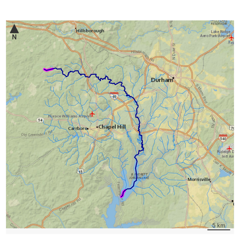 The path extracted above can be reproduced with a network navigation,
which is the more direct path for most applications. Below,
The path extracted above can be reproduced with a network navigation,
which is the more direct path for most applications. Below,
navigate_hydro_network() runs from a starting location,
with the distance parameter limiting how far the navigation
extends from the start point.
# this is just the ids
path <- navigate_hydro_network(hy_net,
start = outlet$id,
mode = "UM")
# filter the source data to get the id's representation
path <- hy_net[hy_net$id %in% path, ]
# pathlength_km is the distance from the furthest downstream network outlet
# it is used within navigate_hydro_network to filter to a given distance.
pathlength <- max(path$pathlength_km) - min(path$pathlength_km)
half_path <- navigate_hydro_network(hy_net,
start = outlet$id,
mode = "UM",
distance = pathlength / 2)
half_path <- hy_net[hy_net$id %in% half_path, ]
par(mar = c(0, 0, 0, 0))
nhdplusTools::plot_nhdplus(bbox = sf::st_bbox(hy_net), plot_config = pc)
plot(map_prep(hy_net), col = "dodgerblue2", add = TRUE, lwd = 0.5)
plot(map_prep(half_path), col = "magenta", add = TRUE, lwd = 3)
plot(map_prep(path), col = "darkblue", add = TRUE, lwd = 2)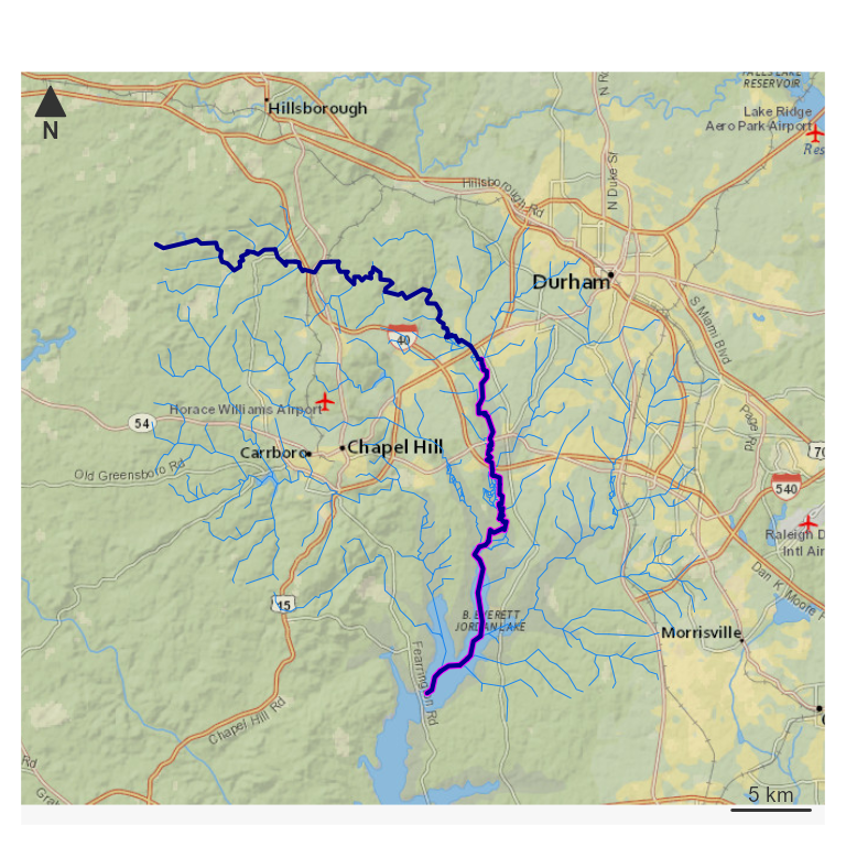 Next, look at
 up and down navigation —
“upstream with tributaries” and “downstream with diversions”, or “UT”
and “DD” in NHDPlus. For this demonstration, the start point is the top
of the half path found above. In practice, the start would be a known
location like a gage site.
start <- half_path[half_path$topo_sort == max(half_path$topo_sort), ]
up <- navigate_hydro_network(hy_net,
start = start$id,
mode = "up")
up <- hy_net[hy_net$id %in% up, ]
down <- navigate_hydro_network(hy_net,
start = start$id,
mode = "down")
down <- hy_net[hy_net$id %in% down, ]
par(mar = c(0, 0, 0, 0))
nhdplusTools::plot_nhdplus(bbox = sf::st_bbox(hy_net), plot_config = pc)
plot(map_prep(hy_net), col = "dodgerblue2", add = TRUE, lwd = 0.5)
plot(map_prep(start), col = "magenta", add = TRUE, lwd = 4)
plot(map_prep(up), col = "darkblue", add = TRUE, lwd = 2)
plot(map_prep(down), col = "blue", add = TRUE, lwd = 2)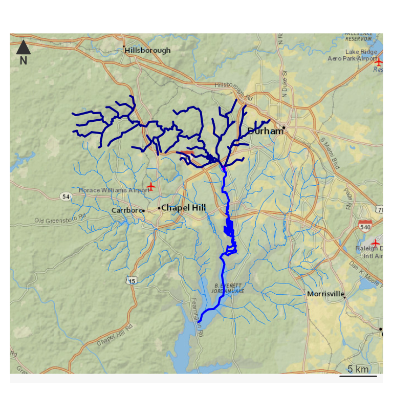 The four navigations above cover most common use cases when the nhdplus
attributes are available. The full nhdplus attribute suite is not always
available, though, and that is where
The four navigations above cover most common use cases when the nhdplus
attributes are available. The full nhdplus attribute suite is not always
available, though, and that is where navigate_network_dfs()
comes in.
Flownetwork-based navigation
navigate_network_dfs() performs up and
down navigation with only a network topology described as
id and toid. If upmain and
downmain attributes are also available, it performs main
path navigation as well.
The definitions of upmain and downmain in
the flow network context are worth a look:
hydroloom_name_definitions[names(hydroloom_name_definitions) == "upmain"]
#>                                                                                      upmain
#> "indicates that a given network element is the primary upstream connection at a confluence"
hydroloom_name_definitions[names(hydroloom_name_definitions) == "downmain"]
#>                                                                                      downmain
#> "indicates that a given network element is the primary downstream connection at a confluence"
Building on the non-dendritic network example from
vignette("hydroloom"), the same five-edge network can carry
upmain and downmain attributes. The network
has one divergence and one confluence. Where id 1 appears
twice it has exactly one downmain == TRUE (the row
connecting to 4), and where toid 5 appears twice it has
exactly one upmain == TRUE (the row from 4). This is the
same divergence case study used in
vignette("non-dendritic"), where it is shown in
hy_node, hy_topo, and
hy_flownetwork form.
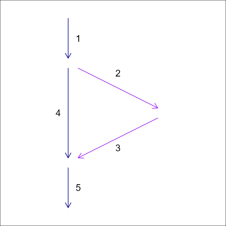
| id | toid | upmain | downmain |
|---|---|---|---|
| 1 | 2 | TRUE | FALSE |
| 1 | 4 | TRUE | TRUE |
| 2 | 3 | TRUE | TRUE |
| 3 | 5 | FALSE | TRUE |
| 4 | 5 | TRUE | TRUE |
| 5 | 0 | TRUE | TRUE |
hydroloom provides utilities to build this lightweight
flownetwork format from a geometric network via
make_attribute_topology(). upmain and
downmain attributes can be constructed using
add_divergence(), add_levelpaths(), and
to_flownetwork(). The sample data already carries
divergence and levelpath attributes, but
reconstructing them is shown below.
# select only id, name, feature_type.
# Note that the geometry is "sticky" and is included in base_net
base_net <- dplyr::select(hy_net, id, GNIS_NAME, feature_type)

# create a geometric network -- this includes divergences
base_net <- dplyr::left_join(make_attribute_topology(base_net, min_distance = 10),
  base_net, by = "id") |>
  sf::st_sf()

names(base_net)
#> [1] "id"           "toid"         "GNIS_NAME"    "feature_type" "geom"
nrow(base_net)
#> [1] 832

# now switch from a flownetwork topology to a node topology.
base_net <- hydroloom::make_node_topology(base_net, add_div = TRUE, add = TRUE)

names(base_net)
#> [1] "id"           "fromnode"     "tonode"       "GNIS_NAME"    "feature_type"
#> [6] "geom"
nrow(base_net)
#> [1] 746

# divergence determination needs a dominant feature type input
unique(base_net$feature_type)
#> [1] "StreamRiver"    "Connector"      "ArtificialPath"

base_net <- add_divergence(base_net,
  coastal_outlet_ids = outlet$id,
  inland_outlet_ids = c(),
  name_attr = "GNIS_NAME",
  type_attr = "feature_type",
  major_types = "StreamRiver")

names(base_net)
#> [1] "id"           "fromnode"     "tonode"       "GNIS_NAME"    "feature_type"
#> [6] "geom"         "divergence"
nrow(base_net)
#> [1] 746

# now we can add a dendritic toid attribute because we have "divergence"
base_net <- add_toids(base_net, return_dendritic = TRUE)

# note that no rows were added -- these are only downmain!
nrow(base_net)
#> [1] 746

# now add a length attribute as the accumulated flowline length.
base_net$length_km <- as.numeric(st_length(base_net) / 1000)
base_net$weight <- accumulate_downstream(base_net, "length_km")
#> Dendritic routing will be applied. Diversions are assumed to have 0 flow fraction.

base_net <- add_levelpaths(base_net,
  name_attribute = "GNIS_NAME",
  weight_attribute = "weight")

names(base_net)
#>  [1] "id"                  "toid"                "levelpath_outlet_id"
#>  [4] "topo_sort"           "levelpath"           "geom"
#>  [7] "tonode"              "GNIS_NAME"           "feature_type"
#> [10] "divergence"          "fromnode"            "length_km"
#> [13] "weight"

# remove dendritic toid used above
base_net <- dplyr::select(base_net, -toid)

flow_net <- to_flownetwork(base_net)

nrow(flow_net)
#> [1] 832
names(flow_net)
#> [1] "id"       "toid"     "upmain"   "downmain"
The pipeline above transforms the data through several
hy subclasses. At each stage,
hy_capabilities() reports which hydroloom functions are
directly callable on the object’s current class and columns. Re-running
the pipeline with intermediate objects makes the progression
visible:
# 1. Raw load -- base hy with geometry only.
step1 <- hy(dplyr::select(hy_net, id, GNIS_NAME, feature_type))
class(step1)
#> [1] "hy"         "sf"         "tbl_df"     "tbl"        "data.frame"
hy_capabilities(step1)
#>               add_toids      make_node_topology          to_flownetwork
#>                   FALSE                   FALSE                   FALSE
#>            sort_network           add_topo_sort          add_levelpaths
#>                   FALSE                   FALSE                   FALSE
#>          add_pathlength         add_streamorder   accumulate_downstream
#>                   FALSE                   FALSE                   FALSE
#>          check_hy_graph  navigate_hydro_network         add_pfafstetter
#>                   FALSE                   FALSE                   FALSE
#>         add_streamlevel          add_divergence   add_return_divergence
#>                   FALSE                   FALSE                   FALSE
#>          subset_network    navigate_network_dfs          make_index_ids
#>                   FALSE                   FALSE                   FALSE
#> make_attribute_topology   index_points_to_lines
#>                    TRUE                    TRUE

# 2. After make_attribute_topology + make_node_topology -- now hy_node.
step2 <- dplyr::left_join(
  make_attribute_topology(step1, min_distance = 10),
  step1, by = "id"
) |>
  sf::st_sf() |>
  make_node_topology(add_div = TRUE, add = TRUE)
class(step2)
#> [1] "hy_node"    "hy"         "sf"         "data.frame"
hy_capabilities(step2)
#>               add_toids      make_node_topology          to_flownetwork
#>                    TRUE                   FALSE                   FALSE
#>            sort_network           add_topo_sort          add_levelpaths
#>                   FALSE                   FALSE                   FALSE
#>          add_pathlength         add_streamorder   accumulate_downstream
#>                   FALSE                   FALSE                   FALSE
#>          check_hy_graph  navigate_hydro_network         add_pfafstetter
#>                   FALSE                   FALSE                   FALSE
#>         add_streamlevel          add_divergence   add_return_divergence
#>                   FALSE                    TRUE                   FALSE
#>          subset_network    navigate_network_dfs          make_index_ids
#>                    TRUE                   FALSE                   FALSE
#> make_attribute_topology   index_points_to_lines
#>                    TRUE                    TRUE

# 3. After add_divergence -- still hy_node, now with divergence so
#    add_return_divergence becomes available.
step3 <- add_divergence(step2,
  coastal_outlet_ids = outlet$id,
  inland_outlet_ids = c(),
  name_attr = "GNIS_NAME",
  type_attr = "feature_type",
  major_types = "StreamRiver")
class(step3)
#> [1] "hy_node"    "sf"         "hy"         "data.frame"
hy_capabilities(step3)
#>               add_toids      make_node_topology          to_flownetwork
#>                    TRUE                   FALSE                   FALSE
#>            sort_network           add_topo_sort          add_levelpaths
#>                   FALSE                   FALSE                   FALSE
#>          add_pathlength         add_streamorder   accumulate_downstream
#>                   FALSE                   FALSE                   FALSE
#>          check_hy_graph  navigate_hydro_network         add_pfafstetter
#>                   FALSE                   FALSE                   FALSE
#>         add_streamlevel          add_divergence   add_return_divergence
#>                   FALSE                    TRUE                    TRUE
#>          subset_network    navigate_network_dfs          make_index_ids
#>                    TRUE                   FALSE                   FALSE
#> make_attribute_topology   index_points_to_lines
#>                    TRUE                    TRUE

# 4. After add_toids(return_dendritic = TRUE) -- promotes to hy_topo,
#    unlocking edge-list operations (sort_network, add_levelpaths,
#    add_streamorder, accumulate_downstream, ...).
step4 <- add_toids(step3, return_dendritic = TRUE)
class(step4)
#> [1] "hy_topo"    "hy"         "sf"         "data.frame"
hy_capabilities(step4)
#>               add_toids      make_node_topology          to_flownetwork
#>                   FALSE                    TRUE                   FALSE
#>            sort_network           add_topo_sort          add_levelpaths
#>                    TRUE                    TRUE                    TRUE
#>          add_pathlength         add_streamorder   accumulate_downstream
#>                    TRUE                    TRUE                    TRUE
#>          check_hy_graph  navigate_hydro_network         add_pfafstetter
#>                    TRUE                    TRUE                   FALSE
#>         add_streamlevel          add_divergence   add_return_divergence
#>                   FALSE                   FALSE                   FALSE
#>          subset_network    navigate_network_dfs          make_index_ids
#>                   FALSE                    TRUE                    TRUE
#> make_attribute_topology   index_points_to_lines
#>                    TRUE                    TRUE

# 5. After add_levelpaths -- promotes to hy_leveled, unlocking
#    add_pfafstetter, add_streamlevel, and to_flownetwork.
step4$length_km <- as.numeric(sf::st_length(step4) / 1000)
step4$weight    <- accumulate_downstream(step4, "length_km")
#> Dendritic routing will be applied. Diversions are assumed to have 0 flow fraction.
step5 <- add_levelpaths(step4,
  name_attribute = "GNIS_NAME",
  weight_attribute = "weight")
class(step5)
#> [1] "hy_leveled" "hy_topo"    "sf"         "hy"         "tbl_df"
#> [6] "tbl"        "data.frame"
hy_capabilities(step5)
#>               add_toids      make_node_topology          to_flownetwork
#>                   FALSE                    TRUE                    TRUE
#>            sort_network           add_topo_sort          add_levelpaths
#>                    TRUE                    TRUE                    TRUE
#>          add_pathlength         add_streamorder   accumulate_downstream
#>                    TRUE                    TRUE                    TRUE
#>          check_hy_graph  navigate_hydro_network         add_pfafstetter
#>                    TRUE                    TRUE                    TRUE
#>         add_streamlevel          add_divergence   add_return_divergence
#>                    TRUE                   FALSE                   FALSE
#>          subset_network    navigate_network_dfs          make_index_ids
#>                   FALSE                    TRUE                    TRUE
#> make_attribute_topology   index_points_to_lines
#>                    TRUE                    TRUE

# 6. After to_flownetwork -- becomes hy_flownetwork; navigate_network_dfs
#    on upmain/downmain is now supported on this lightweight form.
step6 <- to_flownetwork(dplyr::select(step5, -toid))
class(step6)
#> [1] "hy_flownetwork" "tbl_df"         "tbl"            "data.frame"
hy_capabilities(step6)
#>               add_toids      make_node_topology          to_flownetwork
#>                   FALSE                   FALSE                   FALSE
#>            sort_network           add_topo_sort          add_levelpaths
#>                   FALSE                   FALSE                   FALSE
#>          add_pathlength         add_streamorder   accumulate_downstream
#>                   FALSE                   FALSE                   FALSE
#>          check_hy_graph  navigate_hydro_network         add_pfafstetter
#>                   FALSE                   FALSE                   FALSE
#>         add_streamlevel          add_divergence   add_return_divergence
#>                   FALSE                   FALSE                   FALSE
#>          subset_network    navigate_network_dfs          make_index_ids
#>                   FALSE                    TRUE                    TRUE
#> make_attribute_topology   index_points_to_lines
#>                   FALSE                   FALSE
Each transformation either changes the subclass or adds a column that
unlocks additional operations. The progression hy ->
hy_node -> hy_topo ->
hy_leveled -> hy_flownetwork is the
canonical path for working with non-dendritic NHDPlus-like data in
hydroloom.
The result is a flow network. The reconstruction wasn’t strictly
necessary — the demo NHDPlus data already carries every attribute needed
to build one — but it shows how the NHDPlus attributes map onto the
lighter flownetwork attributes. The hydroloom methods are nearly
identical to those of NHDPlus, with minor differences shown below:
nearly all upmain and downmain connections
agree, with a single junction differing.
The difference traces to how the divergence weight is computed.
hydroloom uses dendritic accumulation of flowline length (diversions get
0% of the upstream value) while NHDPlus uses unapportioned accumulation
(diversions get 100% of the upstream value). The resulting
upmain choice at one junction differs by a single
feature.
flow_net_nhdplus <- to_flownetwork(hy_net) |>
  dplyr::arrange(id, toid)

flow_net_hydroloom <- to_flownetwork(base_net) |>
  dplyr::arrange(id, toid)

different_downmain <- flow_net_nhdplus[flow_net_nhdplus$downmain != flow_net_hydroloom$downmain, ]

different_downmain
#> # hydroloom flow network (junction table): 0 connections, 0 diversions
#> # A tibble: 0 × 4
#> # ℹ 4 variables: id <int>, toid <dbl>, upmain <lgl>, downmain <lgl>

different_upmain <- flow_net_nhdplus[flow_net_nhdplus$upmain != flow_net_hydroloom$upmain, ]

different_upmain
#> # hydroloom flow network (junction table): 2 connections, 0 diversions
#> # A tibble: 2 × 4
#>        id    toid upmain downmain
#>     <int>   <dbl> <lgl>  <lgl>
#> 1 8893470 8893552 TRUE   TRUE
#> 2 8893472 8893552 FALSE  TRUE

different_upmain <- hy_net[hy_net$id %in% c(different_upmain$id, different_upmain$toid), ]

par(mar = c(0, 0, 0, 0))
nhdplusTools::plot_nhdplus(bbox = sf::st_bbox(different_upmain), plot_config = pc)
plot(map_prep(hy_net, 10), col = "dodgerblue2", add = TRUE, lwd = 0.5)
plot(map_prep(different_upmain, 10), col = "blue", add = TRUE, lwd = 2)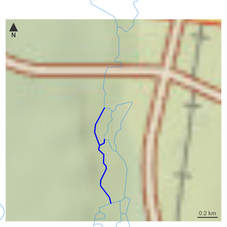
With a flownetwork in hand, the same navigations from earlier can be reproduced — this time using only the basic network, without any NHDPlus attributes.
# this is just the ids
path <- navigate_network_dfs(flow_net,
starts = outlet$id,
direction = "upmain")
# filter the source data to get the id's representation
path <- hy_net[hy_net$id %in% unlist(path), ]
# distance not yet supported
half_path <- navigate_network_dfs(flow_net,
starts = 8893396, # chosen from a map
direction = "downmain")
half_path <- hy_net[hy_net$id %in% unlist(half_path), ]
par(mar = c(0, 0, 0, 0))
nhdplusTools::plot_nhdplus(bbox = sf::st_bbox(hy_net), plot_config = pc)
plot(map_prep(hy_net), col = "dodgerblue2", add = TRUE, lwd = 0.5)
plot(map_prep(half_path), col = "magenta", add = TRUE, lwd = 3)
plot(map_prep(path), col = "darkblue", add = TRUE, lwd = 2)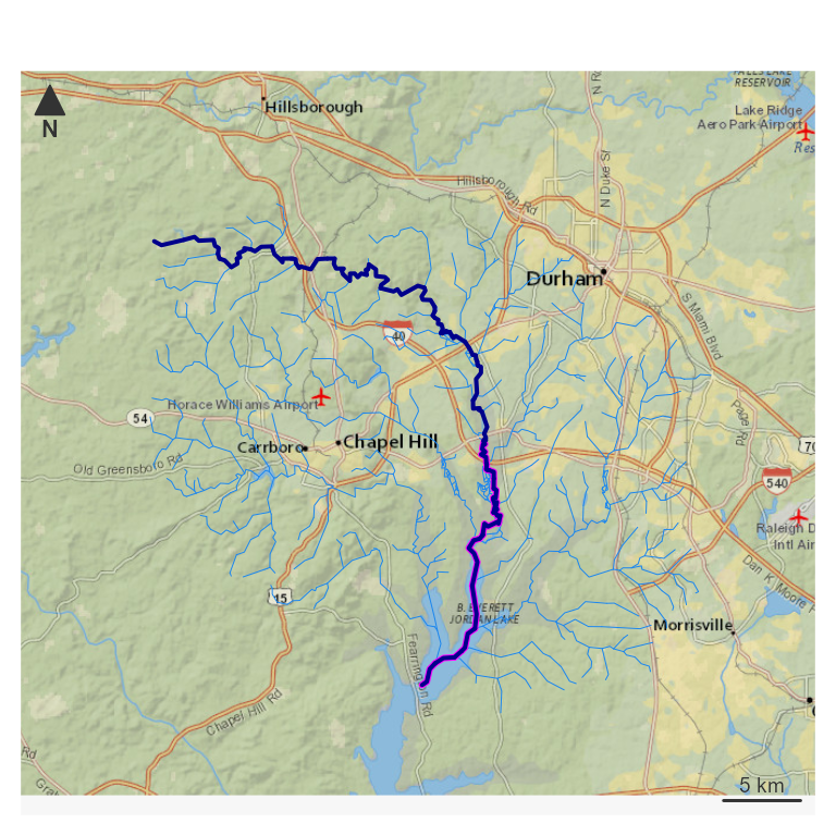 Now look at
 up and down navigation on the
flownetwork. The start point is the same feature picked from the map
above; in practice it would be a known location like a gage site.
# chosen from map
start <- hy_net[hy_net$id == 8893396, ]

up <- navigate_network_dfs(flow_net,
  starts = start$id,
  direction = "up")
up <- hy_net[hy_net$id %in% unlist(up), ]

down <- navigate_network_dfs(flow_net,
  starts = start$id,
  direction = "down")
down <- hy_net[hy_net$id %in% unlist(down), ]

par(mar = c(0, 0, 0, 0))
nhdplusTools::plot_nhdplus(bbox = sf::st_bbox(hy_net), plot_config = pc)
plot(map_prep(hy_net), col = "dodgerblue2", add = TRUE, lwd = 0.5)
plot(map_prep(start), col = "magenta", add = TRUE, lwd = 4)
plot(map_prep(up), col = "darkblue", add = TRUE, lwd = 2)
plot(map_prep(down), col = "blue", add = TRUE, lwd = 2)