Topological Sort Based Network Attributes

Terminology

The terms used below are derived from concepts of graph theory, the HY_Features conceptual data model, and the NHDPlus data model. Many of the concepts here are also presented in: Mainstems: A logical data model implementing mainstem and drainage basin feature types based on WaterML2 Part 3: HY Features concepts. This article formed an early draft of this paper: Generating a reference flow network with improved connectivity to support durable data integration and reproducibility in the coterminous US.

Introduction

The NHDPlus data model, which the attributes described here are based on, includes many ‘value added attributes’ (VAA). This vignette discusses a core set of VAAs that hydroloom can create from readily available hydrographic inputs. The vignette begins with a background needed to understand what these attributes are, and then demonstrates how to create them based on some sample input data. These attributes are documented in the NHDPlus manual, and every effort has been made to faithfully implement their meaning.

While the hydroloom package contains other functions to generate network attributes, (e.g. add_pfafstetter() for Pfafstetter codes and add_streamorder() for stream orders) this vignette focuses on the network attributes from the NHDPlus data model that revolve around the topo_sort and levelpath. In the NHDPlus data model, topo_sort is referred to as hydrosequence but it is functionally equivalent to a topological sort and is referred to as topo_sort in hydroloom.

topo_sort

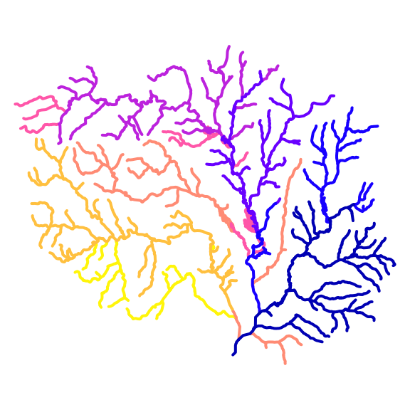
Smaller ‘topo_sort’ values are guaranteed to be downstream of larger values along connected paths.

The NHDPlus data model includes an attribute called hydrosequence that is functionally a topological sort of the flowline network. It provides an integer identifier guaranteed to decrease in the downstream direction. For flowlines that are not connected by a single direction navigation (e.g. parallel tributaries) the topo_sort has no significance. However, when two flowlines have a direct navigation, the downstream flowline will always have the smaller topo_sort. hydroloom supports creation of topo_sort with the sort_network() function.

It is hard to overstate the importance of topo_sort, as any function that requires understanding upstream-downstream relationships requires a sorted version of the flowline network. In the NHDPlus data model, a dendritic edge-list topology is stored in the form of a topo_sort and ‘down topo_sort’ attribute. The equivalent is available in hydroloom, but does not use the to topo_sort convention, preferring the primary identifier (id) and an accompanying toid to store a dendritic edge list.

Level Path

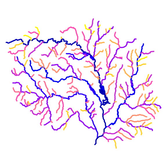
Levelpath values are constant along mainstem paths and are derived from the topo_sort of their outlet flowline.

A level path is derived from “stream level” which assigns an integer value to mainstem rivers from outlet up the network (see NHDPlus documentation for more). Rivers terminating to the ocean are given level 1 and this level extends all the way to the headwaters. Rivers terminating in level 1 rivers are given level 2, and so on.

“Stream leveling” is the process of establishing uniquely identified “level paths” through a stream network. This is accomplished with a set of rules that determine which tributary should be considered dominant at every confluence to establish the “mainstem rivers” for each “drainage basin” in a network. hydroloom supports creation of stream level with the add_streamlevel() function, and the creation of level path with add_levelpaths(). hydroloom adopts the convention used in NHDPlus, to assign the levelpath as the topo_sort of the path’s outlet.

See Mainstems: A logical data model implementing mainstem and drainage basin feature types based on WaterML2 Part 3: HY Features concepts for an in depth discussion of these concepts.

Other Derived Network Attributes

A number of additional attributes can be derived once levelpath and topo_sort are established. These include: (note that precise attribute names have not been used here)

terminal path: the identifier (topo_sort or primary id) of the terminal flowline of network.
up topological sort: the identifier of the upstream flowline on the mainstem
down topological sort: the identifier of the downstream flowline on the mainstem
up level path: the identifier of the next upstream levelpath on the mainstem
down level path: the identifier of the next downstream levelpath on the mainstem
path length: The distance to the network outlet downstream along the main path.
total drainage area: Total accumulated area from upstream flowline’s catchment area.
arbolate sum: The total accumulated length of upstream flowlines.
terminal flag: A simple 0 or 1 indicating whether a flowline is a terminal path or not.

Required Base Attributes

Creating levelpath and topo_sort identifiers requires a set of base attributes that include:

fromnode / tonode or id / toid: from and to nodes can be used to generate an edge to edge flowline topology.
length: a length is required for each flowline in the network to determine a flow distance, and if using the arbolate sum for stream leveling.
area: the local drainage area of each flowline is useful in many contexts but is primarily used to calculate total drainage area.
weight_attribute: a weight metric is required for stream leveling to determine the dominant upstream flowline. In the NHD, the arbolate sum is used. However, alternative metrics (e.g. total drainage area) can be used instead.
name_attribute: Many times, it is preferable to follow a consistently named path rather than a strict physical weight when stream leveling. In these cases a name_attribute can be provided.
divergence: in order to create a [many:1] upstream to downstream topology, diverted paths must be labeled as such. This attribute is 0 for normal (already [many:1]) connections, 1 for the main path through a divergence, and 2 for any diverted path.

A visual introduction to the advanced network attributes

To illustrate the above concepts and attributes, we’ll start with the “New Hope” demo data included in the hydroloom package and add a toid attribute based on the edge-node topology included in the data.

# Import data
x <- hy(sf::read_sf(system.file("extdata/new_hope.gpkg", package = "hydroloom")))

# Strip the data back to the required base attributes
fpath <- hydroloom::add_toids(
  dplyr::select(x, id, fromnode, tonode, divergence, feature_type,
                da_sqkm, length_km, GNIS_ID)
)

# Print
head(fpath <- select(sf::st_cast(fpath, "LINESTRING"), 
                     -tonode, -fromnode, -divergence, -feature_type))
#> Simple feature collection with 6 features and 5 fields
#> Geometry type: LINESTRING
#> Dimension:     XY
#> Bounding box:  xmin: 1517192 ymin: 1555954 xmax: 1518819 ymax: 1557990
#> Projected CRS: +proj=aea +lat_0=23 +lon_0=-96 +lat_1=29.5 +lat_2=45.5 +x_0=0 +y_0=0 +ellps=GRS80 +towgs84=0,0,0,0,0,0,0 +units=m +no_defs
#> # A tibble: 6 × 6
#>        id    toid da_sqkm length_km GNIS_ID                                 geom
#>     <int>   <dbl>   <dbl>     <dbl> <chr>                       <LINESTRING [m]>
#> 1 8893864 8894334  4.81       3.24  991288  (1518702 1557298, 1518643 1557297, …
#> 2 8894490 8894336  0          0.002 991288    (1517194 1556000, 1517192 1555999)
#> 3 8894494 8894490  0.009      0.102 991288  (1517288 1556038, 1517252 1556023, …
#> 4 8894334 8894492  0.428      0.073 991288  (1517349 1556090, 1517341 1556077, …
#> 5 8894492 8894494  0.0018     0.008 991288    (1517295 1556041, 1517288 1556038)
#> 6 8893850 8893864  0.406      0.954 991288  (1518668 1557990, 1518699 1557904, …

topo_sort and terminal ID

After removing attributes used to generate the toid attribute, we have a id and toid relation representing the connectivity of the network as well as attributes required to generate a sorted network with sort_network()

head(fpath <- sort_network(fpath, split = TRUE))
#> Simple feature collection with 6 features and 6 fields
#> Geometry type: LINESTRING
#> Dimension:     XY
#> Bounding box:  xmin: 1505349 ymin: 1554873 xmax: 1508920 ymax: 1558708
#> Projected CRS: +proj=aea +lat_0=23 +lon_0=-96 +lat_1=29.5 +lat_2=45.5 +x_0=0 +y_0=0 +ellps=GRS80 +towgs84=0,0,0,0,0,0,0 +units=m +no_defs
#> # A tibble: 6 × 7
#>        id   toid da_sqkm length_km GNIS_ID terminal_id                      geom
#>     <int>  <dbl>   <dbl>     <dbl> <chr>         <int>          <LINESTRING [m]>
#> 1 8898302 8.90e6   0.152     0.182 "98382…     8897784 (1505349 1555718, 150545…
#> 2 8896658 8.90e6   1.19      1.37  "98382…     8897784 (1505455 1555570, 150547…
#> 3 8896656 8.90e6   3.86      2.64  "98382…     8897784 (1506375 1554873, 150644…
#> 4 8896664 8.90e6   1.38      1.64  " "         8897784 (1507786 1554903, 150781…
#> 5 8896624 8.90e6   1.34      1.17  "98382…     8897784 (1508236 1556343, 150825…
#> 6 8896572 8.90e6   1.56      1.77  " "         8897784 (1508311 1558708, 150835…

The sort_network() function sorts the flowlines such that headwaters come first and the terminal flowline last. Additionally, it produces a terminal_id representing the outlet id of the network. If multiple terminal networks had been provided, the terminal_id would allow us to group the data by complete sub networks (a convenient parallelization scheme).

In contrast to NHDPlus, where the terminal path is identified by the topo_sort id of the outlet flowline (meaning the outlet of a level path is left to a user to generate), hydroloom uses the more stable primary id (COMID in NHDPlus) for identifying outlets to allow the topo_sort attribute to be generated and discarded as needed.

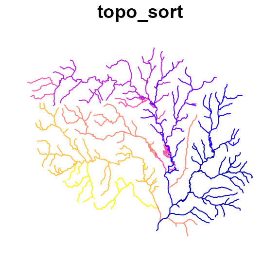
We can visualize this sorting by assigning a temporary “topo_sort” value to the sorted network, row wise. Here, we assign the first rows in the sorted set to large values and the last rows to small values in line with the topo_sort order convention in NHDPlus.

fpath['topo_sort'] <- seq(nrow(fpath), 1)
plot(fpath['topo_sort'], key.pos = NULL)

Level Path and outlet ID

To generate a levelpath attribute, a “physical” weight is needed to determine the upstream mainstem at confluences. For this example, we’ll follow the NHD convention and calculate the arbolate sum explicitly. The add_levelpaths() function will add arbolate sum internally if no weight is explicitly defined.

# Rename and compute weight
fpath$arbolatesum <- accumulate_downstream(
  dplyr::select(fpath, 
                id, toid, length_km), "length_km")

plot(sf::st_geometry(fpath), lwd = fpath$arbolatesum / 10)

A name_attribute identifier can also be provided to override the physical weight_attribute when a “smaller” river has the same name. There is an optional override_factor parameter that signifies if the physical weight is override_factor times (e.g. 5) larger on an unnamed or differently named upstream path, the physical weight will be used in favor of the named id.

# Get levelpaths
fpath <- add_levelpaths(fpath, name_attribute = "GNIS_ID",weight_attribute = "arbolatesum", 
  status = FALSE, override_factor = 5)

# Print
head(fpath)
#> Simple feature collection with 6 features and 10 fields
#> Geometry type: LINESTRING
#> Dimension:     XY
#> Bounding box:  xmin: 1514059 ymin: 1551922 xmax: 1518746 ymax: 1554515
#> Projected CRS: +proj=aea +lat_0=23 +lon_0=-96 +lat_1=29.5 +lat_2=45.5 +x_0=0 +y_0=0 +ellps=GRS80 +towgs84=0,0,0,0,0,0,0 +units=m +no_defs
#> # A tibble: 6 × 11
#>        id    toid levelpath_outlet_id topo_sort levelpath
#>     <int>   <dbl>               <int>     <int>     <dbl>
#> 1 8897784       0             8897784         1         1
#> 2 8894360 8897784             8897784         2         1
#> 3 8894356 8894360             8897784         3         1
#> 4 8894354 8894356             8897784         4         1
#> 5 8894350 8894354             8894350         5         5
#> 6 8893884 8894350             8894350         6         5
#> # ℹ 6 more variables: geom <LINESTRING [m]>, da_sqkm <dbl>, length_km <dbl>,
#> #   GNIS_ID <chr>, terminal_id <int>, arbolatesum <dbl>

plot(fpath["topo_sort"], key.pos = NULL, reset = FALSE)
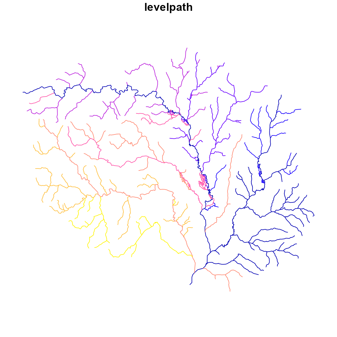
plot(fpath["levelpath"], key.pos = NULL)

Finally, let’s visualize these advanced VAAs!

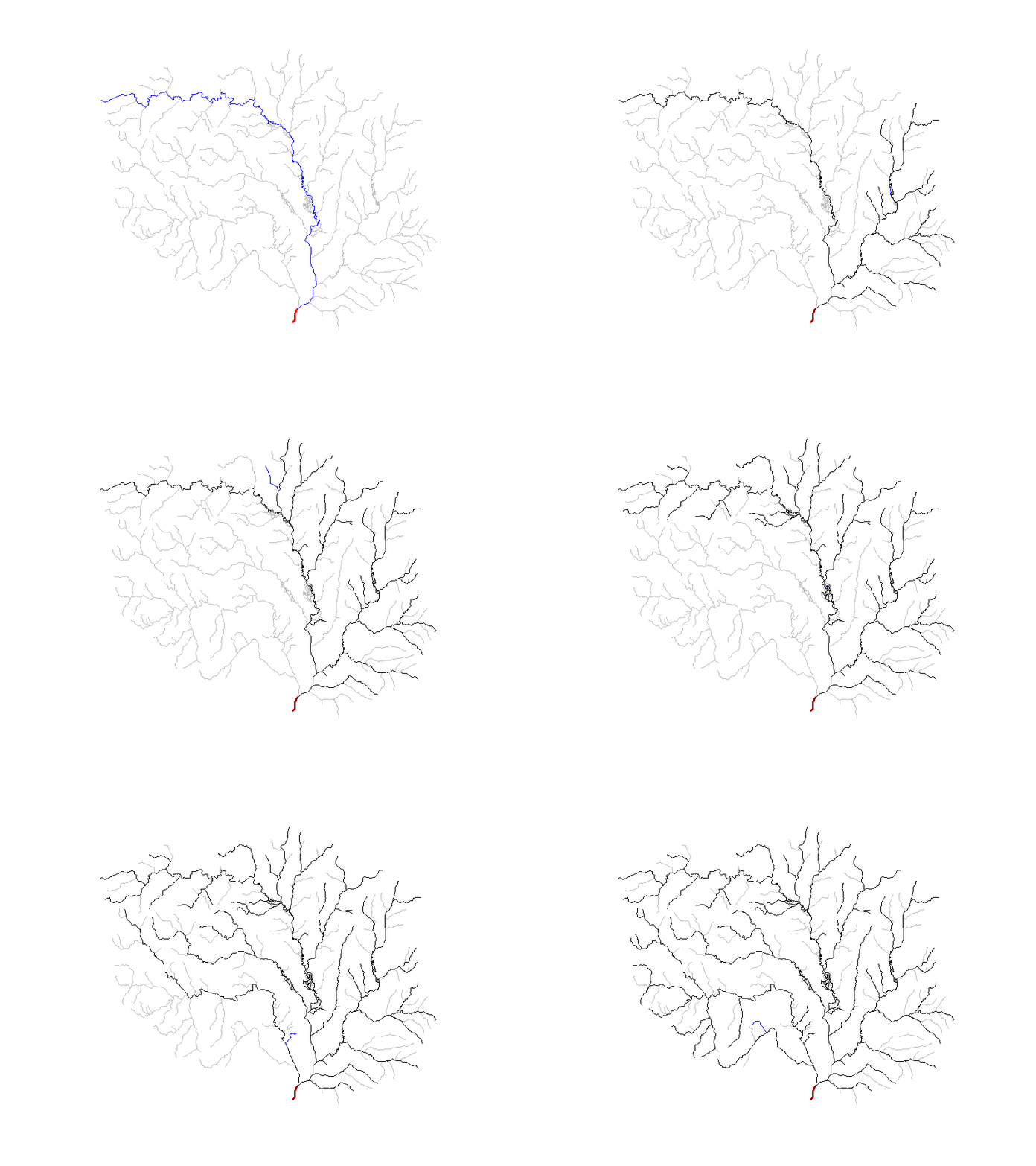
In the below animation, each newly added level path is shown in blue, with the outlet flowline colored in red. Remembering that sort_network() sorts flowlines such that headwaters come first and the terminal flowlines last we invert the network so that level paths fill in from outlet to head waters. For clarity, only levelpaths with more than 2 flowlines are shown.

# Invert plotting order
fpath <- dplyr::arrange(fpath, topo_sort) 

# Level Paths with more then 2 flowlines
lp <- dplyr::group_by(fpath, levelpath) %>%
dplyr::filter(n() > 2) 

# Unique Level Path ID
lp <-  unique(lp$levelpath)

# Terminal flowline 
terminal_fpath <- dplyr::filter(fpath, id %in% terminal_id)

gif_file <- "levelpath.gif"
try({
gifski::save_gif({
  for(i in 1:length(lp)) {
    lp_plot <- dplyr::filter(fpath, levelpath == lp[i])

    outlet_plot <- dplyr::filter(lp_plot, id %in% terminal_id)

    plot(sf::st_geometry(fpath), lwd = 0.5, col = "grey")
    plot(sf::st_geometry(terminal_fpath), lwd = 3, col = "red", add = TRUE)
    plot(sf::st_geometry(dplyr::filter(fpath, levelpath %in% lp[1:i])), add = TRUE)
    plot(sf::st_geometry(lp_plot), col = "blue", add = TRUE)
    plot(sf::st_geometry(outlet_plot), col = "red", lwd = 1.5, add = TRUE)
  }
}, gif_file, delay = 0.5)

knitr::include_graphics(gif_file)
})

Summary

This entire process of sorting the network and building topo_sort, levelpath, and derivative variables is wrapped in the nhdplusTools add_plus_network_attributes function to provide performance and simplicity. It supports parallelization and will print status updates in the case when the input network is very large. add_plus_network_attributes returns NHDPlus attribute names (truncated per shapefile rules as is done in the NHDPlus database).

The attributes described in this vignette assume that diversions in the network have zero flow such that diversions are treated as if they were headwaters. See the vignette("non-dendritic") for information about attributes that include connected divergences.

dblodgett@usgs.gov