Area Weight Generation for Polygon Intersections
Source:vignettes/polygon_intersection.Rmd
polygon_intersection.RmdThis article demonstrates how to create area weights for two sets of polygons.
There are three examples included, one for a typical application with hydrologic units, one for a set of polygons that have gaps and one for polygons without gaps.
Applied Example
It
is a comparison with the gdptools python package
demonstration here.
gdptools_weights <- read.csv(system.file("extdata/gdptools_prl_out.csv", package = "ncdfgeom"),
                             colClasses = c("character", "character", "numeric"))

gdptools_weights <- dplyr::rename(gdptools_weights, gdptools_wght = wght)

gage_id <- "USGS-01482100"
basin <- nhdplusTools::get_nldi_basin(list(featureSource = "nwissite", featureId = gage_id))
huc08 <- nhdplusTools::get_huc(id = na.omit(unique(gdptools_weights$huc8)), type = "huc08")
#> defaulting to 2025 version of WBD
huc12 <- nhdplusTools::get_huc(id = na.omit(unique(gdptools_weights$huc12)), type = "huc12")
#> defaulting to 2025 version of WBD

org_par <- par(mar = c(0, 0, 0, 0))
plot(sf::st_as_sfc(sf::st_bbox(huc12)))
plot(sf::st_geometry(basin), lwd = 4, add = TRUE)
plot(sf::st_simplify(sf::st_geometry(huc08), dTolerance = 500), add = TRUE, lwd = 2)
plot(sf::st_simplify(sf::st_geometry(huc12), dTolerance = 500), add = TRUE, lwd = 0.2, border = "grey")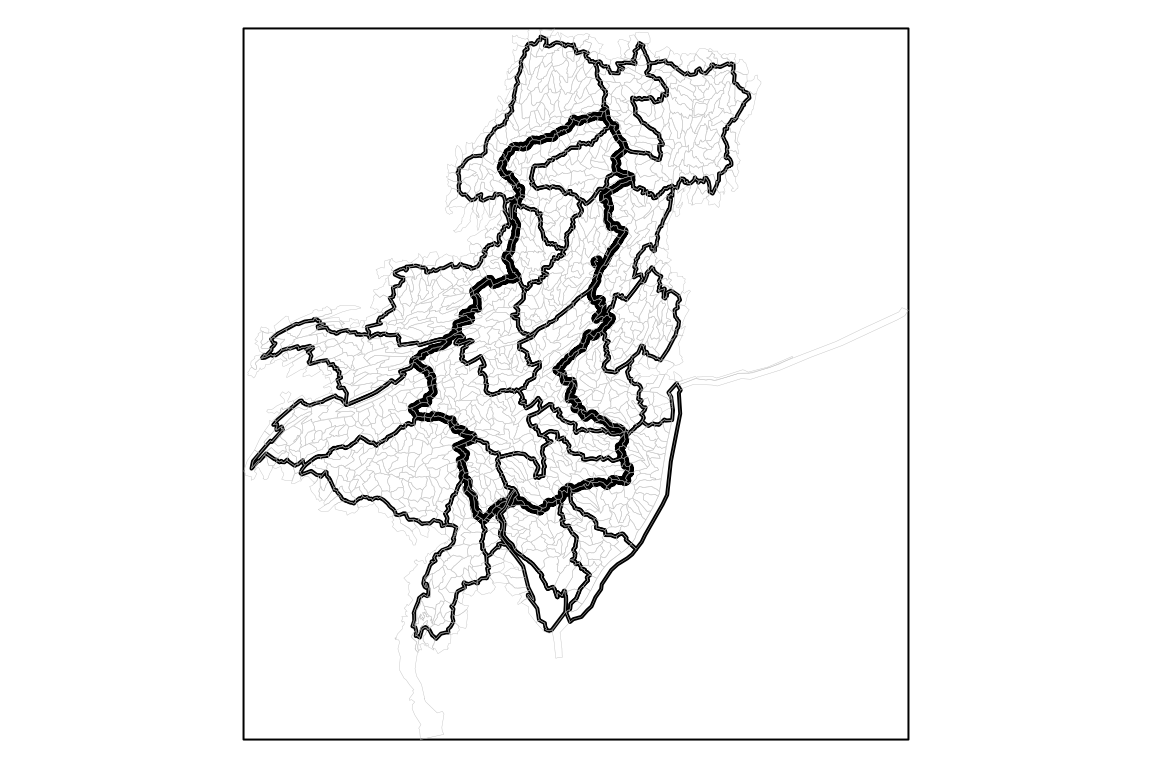
par(org_par)

weights <- ncdfgeom::calculate_area_intersection_weights(
  x = sf::st_transform(dplyr::select(huc12, huc12), 6931),
  y = sf::st_transform(dplyr::select(huc08, huc8), 6931),
  normalize = TRUE
)
#> Loading required namespace: areal

# NOTE: normalize = TRUE means these weights can not be used for "intensive"
# weighted sums such as population per polygon. See below for more on this.

weights <- dplyr::left_join(weights, gdptools_weights, by = c("huc8", "huc12"))
With weights calculated, we can do a little investigation into the differences.
weights$diff <- weights$w - weights$gdptools_wght

# make sure nothing is way out of whack
max(weights$diff, na.rm = TRUE)
#> [1] 0.0005182665

# ensure the weights generally sum as we would expect.
sum(weights$gdptools_wght, na.rm = TRUE)
#> [1] 25
sum(weights$w, na.rm = TRUE)
#> [1] 25
length(unique(na.omit(weights$huc8)))
#> [1] 25

# see how many NA values we have in each.
sum(is.na(weights$w))
#> [1] 182
sum(is.na(weights$gdptools_wght))
#> [1] 182

# look at cases where gptools has NA and ncdfgeom does not
weights[is.na(weights$gdptools_wght) & !is.na(weights$w),]
#> # A tibble: 0 × 5
#> # ℹ 5 variables: huc12 <chr>, huc8 <chr>, w <dbl>, gdptools_wght <dbl>,
#> #   diff <dbl>
Extended Example One
The following example illustrates the nuances between normalized and non-normalized area weights and shows more specifically how area weight intersection calculations can be accomplished for both intensive variables, like total population, and extensive variables, like average precipitation depth.
The set of polygons are a contrived but useful for the sake of demonstration.
library(dplyr)
#>
#> Attaching package: 'dplyr'
#> The following objects are masked from 'package:stats':
#>
#>     filter, lag
#> The following objects are masked from 'package:base':
#>
#>     intersect, setdiff, setequal, union
library(sf)
#> Warning: package 'sf' was built under R version 4.5.3
#> Linking to GEOS 3.14.1, GDAL 3.12.1, PROJ 9.7.1; sf_use_s2() is TRUE
library(ncdfgeom)

g <- list(rbind(c(-1,-1), c(1,-1), c(1,1), c(-1,1), c(-1,-1)))

blue1 = sf::st_polygon(g) * 0.8
blue2 = blue1 + c(1, 2)
blue3 = blue1 * 1.2 + c(-1, 2)

pink1 = sf::st_polygon(g)
pink2 = pink1 + 2
pink3 = pink1 + c(-0.2, 2)
pink4 = pink1 + c(2.2, 0)

blue = sf::st_sfc(blue1,blue2,blue3)

pink = sf::st_sfc(pink1, pink2, pink3, pink4)

plot(c(blue,pink), border = NA)
plot(blue, border = "#648fff", add = TRUE)
plot(pink, border = "#dc267f", add = TRUE)

blue <- sf::st_sf(blue, data.frame(idblue = c(1, 2, 3)))
pink <- sf::st_sf(pink, data.frame(idpink = c(7, 8, 9, 10)))

text(sapply(sf::st_geometry(blue), \(x) mean(x[[1]][,1]) + 0.4),
     sapply(sf::st_geometry(blue), \(x) mean(x[[1]][,2]) + 0.3),
     blue$idblue, col = "#648fff")

text(sapply(sf::st_geometry(pink), \(x) mean(x[[1]][,1]) + 0.4),
     sapply(sf::st_geometry(pink), \(x) mean(x[[1]][,2])),
     pink$idpink, col = "#dc267f")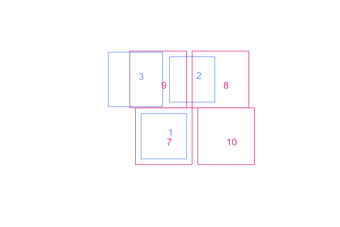
sf::st_agr(blue) <- sf::st_agr(pink) <- "constant"
sf::st_crs(pink) <- sf::st_crs(blue) <- sf::st_crs(5070)
Here, we compare blue (source) and pink (target) and w is the
fraction of blue (source) that is covered pink (target) since we set
normalize = FALSE.
(blue_pink_norm_false <-
calculate_area_intersection_weights(blue, pink, normalize = FALSE))
#> # A tibble: 4 × 3
#>   idblue idpink     w
#>    <dbl>  <dbl> <dbl>
#> 1      1      7 1
#> 2      2      8 0.5
#> 3      2      9 0.375
#> 4      3      9 0.604
NOTE: normalize = FALSE so weights sum to 1 per
source polygon only when a source polygon is fully covered by
the target. The non-intersecting portion is not included.
The following breaks down how to use these weights for intensive or extensive variables.
blue$val = c(30, 10, 20)
blue$area_blue <- as.numeric(sf::st_area(blue))

(result <- st_drop_geometry(blue) |>
  left_join(blue_pink_norm_false, by = "idblue"))
#>   idblue val area_blue idpink         w
#> 1      1  30    2.5600      7 1.0000000
#> 2      2  10    2.5600      8 0.5000000
#> 3      2  10    2.5600      9 0.3750000
#> 4      3  20    3.6864      9 0.6041667
For intensive variables, such as precipitation depth, to calculate the value for pink-9, we calculate an area-weighted mean:
((10 * 0.375 * 2.56) + (20 * 0.604167 * 3.6864)) / ((0.375 * 2.56) + (0.604167 * 3.6864))
#> [1] 16.98795
This is saying that 0.375 of blue-3 covers pink-9 and 0.6 of blue-2 covers pink-9. Since we are calculating a area weighted mean for an intensive variable, we multiply the fraction of each source polygon by its area and the value we want to create an area weight for. We sum the contributions from blue-2 and blue-3 to pink-9 and divide by the sum of the combined area weights.
NOTE: Because there is no contribution to pink-9 over some parts of the polygon, that missing area does not appear. The intersecting areas are 0.96 and 2.23 meaning that we are missing
4 - 0.96 - 2.23 = 0.81
and could rewrite the value for pink-9 as:
((10 * 0.375 * 2.56) + (20 * 0.604167 * 3.6864)) + (NA * 1 * 0.81) /
  ((1 * 0.81) + (0.375 * 2.56) + (0.604167 * 3.6864))
#> [1] NA
Which evaluates to NA. This is why for this operation we usually drop NA terms!
For extensive variables, such as population, to calculate the value of pink-9 we would do:
((10 * 0.375) + (20 * 0.604167))
#> [1] 15.83334
This is saying that 0.375 of blue-3 covers pink-9 and 0.6 of blue-2 covers pink-9. Since we are apportioning the counts of an intensive variable from blue to pink, the weight can be used directly without calculating an area weighted mean.
In practice, the above can be accomplished with
dplyr::group_by() and dplyr::summarize()
(result <- result |>
  group_by(idpink) |> # group so we get one row per target
  # now we calculate the value for each `pink` with fraction of the area of each
  # polygon in `blue` per polygon in `pink` with an equation like this:
  summarize(
    new_val_intensive = sum((val * w * area_blue)) / sum(w * area_blue),
    new_val_extensive = sum(val * w)))
#> # A tibble: 3 × 3
#>   idpink new_val_intensive new_val_extensive
#>    <dbl>             <dbl>             <dbl>
#> 1      7              30                30
#> 2      8              10                 5
#> 3      9              17.0              15.8
Now let’s do the same thing but with normalize = TRUE.
In this case, area is built into w so you
don’t need to know it when using w for intensive variables.
The downfall with normalized weights is that they can not be used
directly with extensive variables.
Here, we set blue as source and pink as target as was done above but
change normalize to TRUE.
(blue_pink_norm_true <-
calculate_area_intersection_weights(select(blue, idblue), pink, normalize = TRUE))
#> # A tibble: 4 × 3
#>   idblue idpink     w
#>    <dbl>  <dbl> <dbl>
#> 1      1      7 0.64
#> 2      2      8 0.32
#> 3      2      9 0.24
#> 4      3      9 0.557
NOTE: normalize = TRUE so weights sum to 1 per target polygon. Non-overlap is ignored as if it does not exist.
The following breaks down how to use these weights for intensive variables.
(result <- st_drop_geometry(blue) |>
    left_join(blue_pink_norm_true, by = "idblue"))
#>   idblue val area_blue idpink      w
#> 1      1  30    2.5600      7 0.6400
#> 2      2  10    2.5600      8 0.3200
#> 3      2  10    2.5600      9 0.2400
#> 4      3  20    3.6864      9 0.5568
To calculate the area weighted mean value for pink-9, we would do:
((10 * 0.24) + (20 * 0.5568)) / (0.24 + (0.5568))
#> [1] 16.98795
This is saying that the portion of pink-9 that should get the value from blue-2 is 0.3 and the portion of pink-9 that should get the value from blue-3 is 0.7. In this form, our weights include the relative area of the source polygons.
As shown above as well, the calculation can be accomplished with:
(result <- result |>
    group_by(idpink) |> # group so we get one row per target
    # now we calculate the value for each `pink` with fraction of the area of each
    # polygon in `blue` per polygon in `pink` with an equation like this:
    summarize(
      new_val = sum((val * w)) / sum(w)))
#> # A tibble: 3 × 2
#>   idpink new_val
#>    <dbl>   <dbl>
#> 1      7    30
#> 2      8    10
#> 3      9    17.0
Extended Example Two
We can look at a more typical arrangement of polygons and look at this a different way. The following polygons are used below to illustrate transferring data from one set of polygons to another.
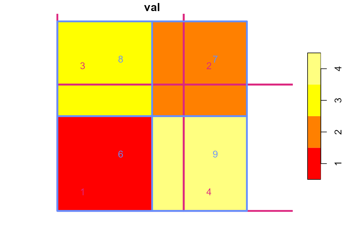
Let’s also look at the values.

In the example code below, values from blue are translated to values from pink using two methods: an weighted sum is done for extensive data such as population data and a weighted mean is done for intensive data such as precipitation depth.
# say we have data from `blue` that we want sampled to `pink`.
# this gives the percent of each `blue` that intersects each `pink`

(blue_pink <- calculate_area_intersection_weights(
  select(blue, idblue), select(pink, idpink), normalize = FALSE))
#> # A tibble: 9 × 3
#>   idblue idpink     w
#>    <dbl>  <dbl> <dbl>
#> 1      6      1 1
#> 2      7      1 0.111
#> 3      8      1 0.333
#> 4      9      1 0.333
#> 5      7      2 0.444
#> 6      7      3 0.222
#> 7      8      3 0.667
#> 8      7      4 0.222
#> 9      9      4 0.667

# NOTE: `w` sums to 1 per `blue` in all cases

summarize(group_by(blue_pink, idblue), w = sum(w))
#> # A tibble: 4 × 2
#>   idblue     w
#>    <dbl> <dbl>
#> 1      6     1
#> 2      7     1
#> 3      8     1
#> 4      9     1

# Since normalize is false, we apply weights like:
st_drop_geometry(blue) |>
  left_join(blue_pink, by = "idblue") |>
  group_by(idpink) |> # group so we get one row per `pink`
  # now we calculate the value for each `pink` with fraction of the area of each
  # polygon in `blue` per polygon in `pink` with an equation like this:
  summarize(
    new_val_intensive = sum( (val * w * blue_areasqkm) ) / sum(w * blue_areasqkm),
    new_val_extensive = sum( (val * w) ))
#> # A tibble: 4 × 3
#>   idpink new_val_intensive new_val_extensive
#>    <dbl>             <dbl>             <dbl>
#> 1      1              2                3.56
#> 2      2              2                0.889
#> 3      3              2.75             2.44
#> 4      4              3.5              3.11

# NOTE: `w` is the fraction of the polygon in `blue`. We need to multiply `w` by the
# unique area of the polygon it is associated with to get the weighted mean weight.

# we can go in reverse if we had data from `pink` that we want sampled to `blue`

(pink_blue <- calculate_area_intersection_weights(
  select(pink, idpink), select(blue, idblue), normalize = FALSE))
#> # A tibble: 9 × 3
#>   idpink idblue      w
#>    <dbl>  <dbl>  <dbl>
#> 1      1      6 0.562
#> 2      1      7 0.0625
#> 3      2      7 0.25
#> 4      3      7 0.125
#> 5      4      7 0.125
#> 6      1      8 0.188
#> 7      3      8 0.375
#> 8      1      9 0.188
#> 9      4      9 0.375

# NOTE: `w` sums to 1 per `pink` (source) only where `pink` is fully covered by `blue` (target).

summarize(group_by(pink_blue, idpink), w = sum(w))
#> # A tibble: 4 × 2
#>   idpink     w
#>    <dbl> <dbl>
#> 1      1  1
#> 2      2  0.25
#> 3      3  0.5
#> 4      4  0.5

# Now let's look at what happens if we set normalize = TRUE. Here we
# get `blue` as source and `pink` as target but normalize the weights so
# the area of `blue` is built into `w`.

(blue_pink <- calculate_area_intersection_weights(
  select(blue, idblue), select(pink, idpink), normalize = TRUE))
#> # A tibble: 9 × 3
#>   idblue idpink      w
#>    <dbl>  <dbl>  <dbl>
#> 1      6      1 0.562
#> 2      7      1 0.0625
#> 3      8      1 0.188
#> 4      9      1 0.188
#> 5      7      2 0.25
#> 6      7      3 0.125
#> 7      8      3 0.375
#> 8      7      4 0.125
#> 9      9      4 0.375

# NOTE: if we summarize by `pink` (target) `w` sums to 1 only where there is full overlap.

summarize(group_by(blue_pink, idpink), w = sum(w))
#> # A tibble: 4 × 2
#>   idpink     w
#>    <dbl> <dbl>
#> 1      1  1
#> 2      2  0.25
#> 3      3  0.5
#> 4      4  0.5

# Since normalize is false, we apply weights like:
st_drop_geometry(blue) |>
  left_join(blue_pink, by = "idblue") |>
  group_by(idpink) |> # group so we get one row per `pink`
  # now we weight by the percent of each polygon in `pink` per polygon in `blue`
  summarize(new_val = sum( (val * w) ) / sum( w ))
#> # A tibble: 4 × 2
#>   idpink new_val
#>    <dbl>   <dbl>
#> 1      1    2
#> 2      2    2
#> 3      3    2.75
#> 4      4    3.5

# NOTE: `w` is the fraction of the polygon from `blue` overlapping the polygon from `pink`.
# The area of `blue` is built into the weight so we just sum the with times value per polygon.
# We can not calculate intensive weighted sums with this weight.