Domain decomposition

dblodgett@usgs.gov

Domains and the extensive connectivity

decompose_network() partitions a hydrologic network into independent sub-basins called domains and stores each basin’s regionally-connecting flowlines separately as the basin’s extensive network — the features that realize its extensive connectivity. Every hy_domain is functionally the same: a self-contained piece of one drainage basin, holding the segment’s lateral tributaries together with the extensive network rows that flow through the segment.

The extensive network is the basin’s connecting flowlines with their toids intact — a hy_leveled view, addressable end-to-end for drawing, naming, or any operation that wants the full network. The extensive network rows that appear in the overlay also appear inside the domains, but with their toids set to the reserved outlet value returned by get_outlet_value(). Each becomes a local outlet of its own contributing sub-basin.

The duplication is deliberate. With the same rows held both ways, a domain’s accumulation runs as a single pass over its catchments and the basin’s extensive network stays queryable as one object. Editing or re-attributing a single domain does not invalidate any other.

Use case

A catchment network covering a large area carries many features with upstream-downstream dependencies. decompose_network() splits such a network into self-contained sub-basins so that each domain can be processed independently, then recomposed into a single result.

In practice, this gives three things:

• A domain’s catchment network is self-contained, so per-domain processing can be run in parallel.
• Recomposition is a single pass through the inter-domain graph derived from the nexus registry. Per-domain results combine through the basin’s extensive network to produce basin-wide answer.
• Editing is decoupled. A new modeled result, a corrected geometry, or a re-derived attribute lands in one domain at a time, and the basin catches up by replaying recomposition.

Decomposed and recomposed modes

A domain’s catchments slot holds two kinds of rows: the lateral tributary rows and the extensive network rows that flow through the domain’s segment. On the extensive network rows, the toid is set to the reserved outlet value returned by get_outlet_value(), so each becomes a local outlet of its own contributing sub-basin. This is the decomposed mode — the default form decompose_network() returns. Extensive network membership inside a domain is recoverable by intersecting the domain’s catchments$id with the basin’s extensive network overlay’s id.

In decomposed mode a single accumulate_downstream() call on a domain’s catchments produces, for every extensive network row, the locally-incremental drainage area (or any other accumulable) belonging there: the row’s own incremental plus the lateral tributaries that drain into it. Per-domain processing is independent and runs in parallel.

To switch to recomposed mode, restore the extensive network rows’ toids from source_network:

restored <- domain$catchments
src_lookup <- setNames(source_network$toid, source_network$id)
outlet_value <- get_outlet_value(restored)
detoid_idx <- which(restored$toid == outlet_value)
restored$toid[detoid_idx] <- src_lookup[as.character(restored$id[detoid_idx])]

The domain’s segment is now a connected sub-basin again; standard hydroloom operations (model coupling, hydraulic routing, end-to-end visualization) work unchanged. Switching back is a one-column assignment.

Functional characteristics

The decomposition operates on drainage basins. A drainage basin is the total upstream area draining to an outlet, with a single mainstem connecting its headwater to that outlet. The input network may contain one or more drainage basins, each composed of incremental catchments connected in an upstream-downstream topology.

For each drainage basin, decompose_network() identifies the basin’s extensive network — the outlet levelpath by default, or the union of levelpaths whose outlet metric exceeds stem_threshold — and divides it into segments at confluences. Each segment becomes a domain whose catchments slot holds the lateral tributaries draining into the segment together with the segment’s extensive network rows in their decomposed form. Even segments with no lateral tributaries become domains — the extensive network rows alone constitute the segment’s contributing area.

The basin’s extensive network overlay is built alongside the domains. It is a hy_leveled view of the same connecting flowlines, with toids intact, so the connected mainstem is addressable end-to-end. The same rows appear in their decomposed form across the segment domains.

A domain corresponds to an HY_Features catchment aggregate. Its drainage area is the full contributing area to its segment. The decomposition does not materialize catchment aggregate objects directly; the alignment is by construction, with the domain’s catchments slot holding the rows the aggregate would.

The inter-domain graph records flow between domains through synthetic nexus identifiers, with one edge per inter-segment handoff. The graph is derived on demand from nexus_registry; see get_domain_graph().

Separation of concerns

The decomposition separates two concerns:

1. Per-domain computation. Each domain’s catchment network is self-contained. Processing a domain requires no information from any other domain beyond what arrives at inlet nexuses.
2. Inter-domain connectivity. The derived domain graph captures which domains flow into which, and at what nexus — a coarser-resolution network that can be traversed independently of catchment-level detail.

Data model

The decomposition produces a domain_decomposition object with six slots:

• domains — named list of hy_domain objects, one per sub-basin segment.
• domain_connectivity — named list of hy_leveled overlays keyed by basin id. Each overlay is the basin’s extensive network: a hy_leveled view of the connecting flowlines with toids intact except at the basin outlet, which carries the reserved outlet toid value. Sub-threshold basins have no overlay.
• overrides — non-dendritic inter-domain transfer table, or NULL.
• catchment_domain_index — named character vector mapping each catchment id to its domain id.
• nexus_registry — synthetic nexus identifiers and the domains they connect.
• source_network — the original enriched input network.

The inter-domain edge list is not stored; get_domain_graph() derives it from nexus_registry on demand.

hy_domain

A hy_domain bundles a domain’s catchment network with the connectivity metadata that recomposition needs:

• domain_id — unique identifier.
• outlet_nexus_id — the hydro nexus where this domain discharges.
• inlet_nexus_ids — hydro nexus ids where upstream domains feed into this one. character(0) for leaf domains; populated for stem and root domains.
• containing_domain_id — the enclosing domain for endorheic basins, or NA.
• catchments — hydroloom object carrying the domain’s catchment network. Catchments include both lateral tributary rows and the segment’s extensive network rows; the extensive network rows have a toid set to get_outlet_value(). To tell the two apart, intersect the domain’s catchments$id with the basin’s extensive network overlay’s id.

The catchments slot accepts hy_topo, hy_leveled, or hy_flownetwork.

S3 classes

The decomposition builds on the hydroloom S3 class hierarchy described in vignette("hydroloom"). The relevant classes are:

• hy_topo — self-referencing edge list (id, toid; unique id).
• hy_leveled — subclass of hy_topo enriched with topo_sort, levelpath, and levelpath_outlet_id. Required input for decompose_network(), because the partition uses levelpath to identify extensive network membership and topo_sort to establish processing order.
• hy_flownetwork — non-dendritic edge list (id, toid; non-unique id allowed). Domains may hold hy_flownetwork catchments to preserve internal divergences.

Running a decomposition

The input must be enriched to hy_leveled before decomposition. add_toids() and add_levelpaths() handle the topology and levelpath enrichment; add_streamorder() adds the stream_calculator column that decompose_network() consults when stem_threshold is supplied (see Extensive Network selection below). For data carrying a StreamCalc column from NHDPlus, the column is already canonicalized by hy() to stream_calculator, so skip add_streamorder(); for other sources it is required.

library(hydroloom)

g <- sf::read_sf(system.file("extdata/new_hope.gpkg", package = "hydroloom"))

src <- hy(g) |>
  add_toids(return_dendritic = TRUE) |>
  add_levelpaths(name_attribute = "GNIS_ID",
    weight_attribute = "arbolate_sum")

d <- decompose_network(src)

The returned domain_decomposition prints a summary of the partition:

d
#> <domain_decomposition: 1 basins, 1 domains, 746 catchments>
#>   domains:              1
#>   domain_connectivity:  1 basins
#>   nexus_registry:       1 nexuses
#>   overrides:            0 rows
#>   source_network:       746 catchments
#> 
#> # Use print(x, full = TRUE) for the full tree summary

Extensive Network selection

decompose_network() determines which catchments carry the basin’s extensive network through one of three paths:

• Default (both stem_threshold and stem_levelpaths are NULL) — the extensive network is the basin’s outlet levelpath.
• Threshold-based — when stem_threshold is supplied, a basin’s outlet metric must exceed the threshold for the basin to be split along its extensive network. Sub-threshold basins become a single domain with no extensive network overlay.
• Explicit — when stem_levelpaths is supplied, those levelpaths (plus the outlet levelpath) form the extensive network.

d_thresh <- decompose_network(src, stem_threshold = 100)

d_thresh
#> <domain_decomposition: 1 basins, 4 domains, 746 catchments>
#>   domains:              4
#>   domain_connectivity:  1 basins
#>   nexus_registry:       4 nexuses
#>   overrides:            0 rows
#>   source_network:       746 catchments
#> 
#> # Use print(x, full = TRUE) for the full tree summary

The map below colors each flowline by the domain it belongs to and overlays the basin’s extensive network in black. Every flowline belongs to some domain (the partition covers the network); the overlay highlights the rows that are also in the basin’s extensive network — the connecting flowlines that the domains turn into local outlets.

# Build a domain_id column on the source flowlines.
domain_idx <- d_thresh$catchment_domain_index
plot_net <- d_thresh$source_network
plot_net$domain_id <- unname(domain_idx[as.character(plot_net$id)])

# Pull all extensive network ids from every basin's overlay.
conn_ids <- unlist(lapply(d_thresh$domain_connectivity,
  \(o) as.character(o$id)),
  use.names = FALSE)

domain_ids <- sort(unique(plot_net$domain_id))

set.seed(42)
pal <- sample(grDevices::hcl.colors(length(domain_ids), palette = "Set 2"))
names(pal) <- domain_ids

par(mar = c(0, 0, 1, 0))
plot(sf::st_geometry(plot_net),
  col = pal[plot_net$domain_id],
  lwd = 2, main = "Domain decomposition (stem_threshold = 100)")
plot(sf::st_geometry(plot_net[as.character(plot_net$id) %in% conn_ids, ]),
  col = "black", lwd = 2, add = TRUE)
legend("topright", legend = c("extensive network overlay",
  "domain (each color = one)"),
  col = c("black", "grey60"), lwd = 2, bty = "n", cex = 0.8)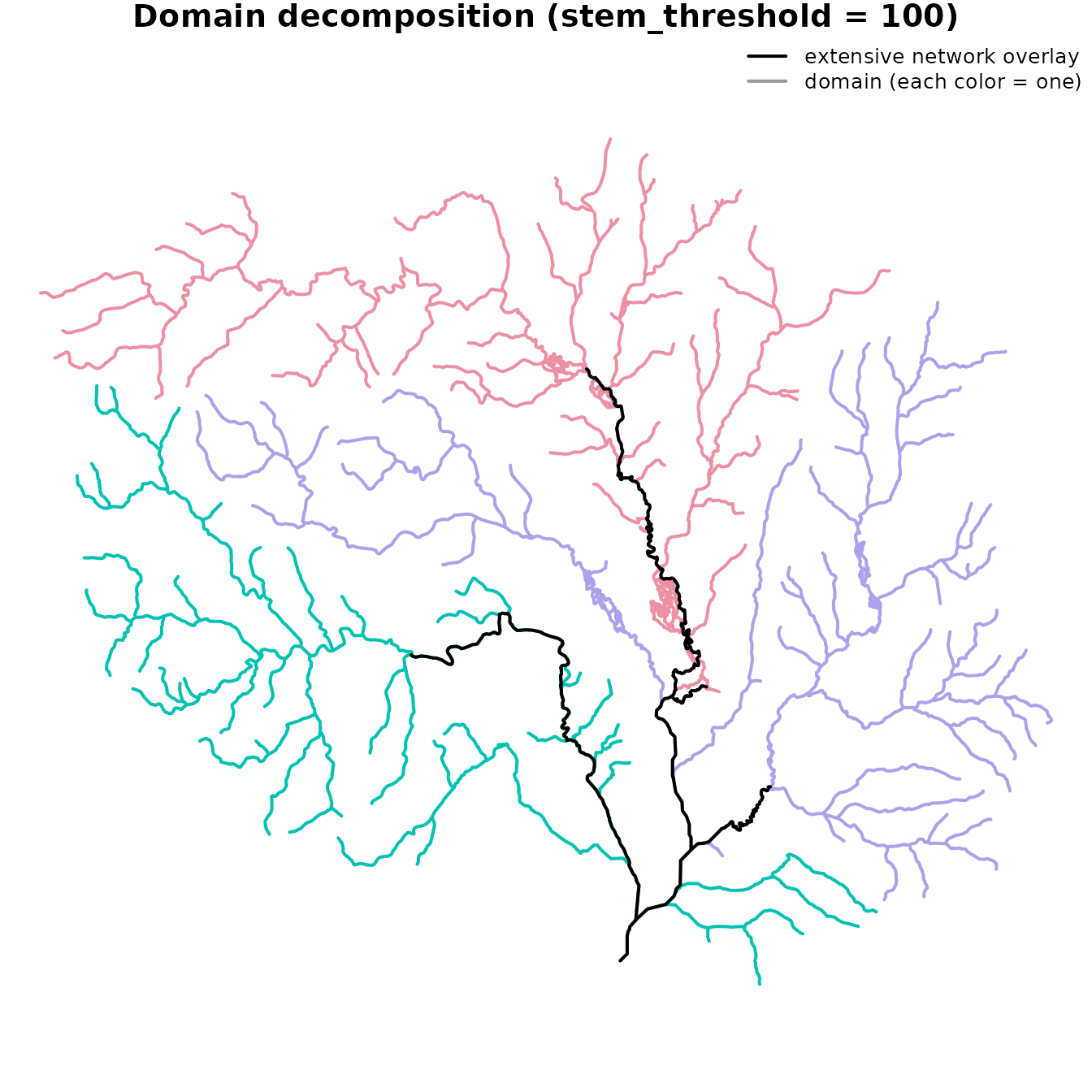

Manual domain breaks

The automatic segmentation splits at confluences — every point where a tributary enters starts a new segment. A large threshold pulls more rivers into domains producing fewer, larger domains. The domain_breaks parameter gives direct control over where the network is segmented, independent of the confluence structure.

In practice, this is useful when domain boundaries need to align with modeling sub-basins, gauge locations, or administrative units rather than the topology’s natural confluence points. The approach is to set a high threshold and then pass specific catchment ids as break points.

# A high threshold pulls many levelpaths into the extensive network.
# Without domain_breaks the extensive network is segmented at every
# confluence, which may produce more domains than desired.
d_high <- decompose_network(src, stem_threshold = 25)
d_high
#> <domain_decomposition: 1 basins, 9 domains, 746 catchments>
#>   domains:              9
#>   domain_connectivity:  1 basins
#>   nexus_registry:       9 nexuses
#>   overrides:            0 rows
#>   source_network:       746 catchments
#> 
#> # Use print(x, full = TRUE) for the full tree summary

# Identify extensive network catchments where we want to force segment
# boundaries. Here we pick two catchments roughly in the middle of
# the extensive network overlay.
conn <- d_high$domain_connectivity[[1]]

# Choose break points at the 1/3 and 2/3 marks along the extensive
# network.
break_ids <- conn$id[
  c(floor(nrow(conn) / 3), floor(2 * nrow(conn) / 3))]

d_manual <- decompose_network(src,
  stem_threshold = 25,
  domain_breaks = break_ids)
d_manual
#> <domain_decomposition: 1 basins, 11 domains, 746 catchments>
#>   domains:              11
#>   domain_connectivity:  1 basins
#>   nexus_registry:       11 nexuses
#>   overrides:            0 rows
#>   source_network:       746 catchments
#> 
#> # Use print(x, full = TRUE) for the full tree summary

The map below compares the automatic segmentation (left) with the manual-break segmentation (right). Both use the same threshold; the difference is where domains attach along the extensive network.

plot_decomp <- function(d, title) {

  domain_idx <- d$catchment_domain_index
  net <- d$source_network
  net$domain_id <- unname(domain_idx[as.character(net$id)])

  conn_ids <- unlist(lapply(d$domain_connectivity,
    \(o) as.character(o$id)),
    use.names = FALSE)

  domain_ids <- sort(unique(net$domain_id))

  set.seed(42)
  pal <- sample(grDevices::hcl.colors(
    max(length(domain_ids), 1), palette = "Set 2"))
  names(pal) <- domain_ids

  plot(sf::st_geometry(net),
    col = pal[net$domain_id],
    lwd = 2, main = title)
  plot(sf::st_geometry(net[as.character(net$id) %in% conn_ids, ]),
    col = "black", lwd = 2, add = TRUE)

}

par(mfrow = c(1, 2), mar = c(0, 0, 2, 0))
plot_decomp(d_high, "Automatic segmentation")
plot_decomp(d_manual, "Manual domain_breaks")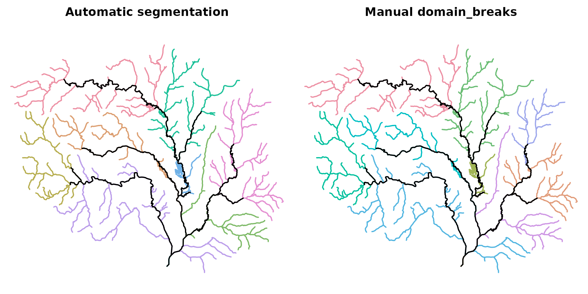

Recomposition

recompose(decomposition, var) accumulates a numeric variable on source_network through the decomposed fabric and returns the source network with the per-row downstream-accumulated value populated.

The function runs in two passes. Pass 1 calls accumulate_downstream() on each domain — the lateral rows roll up within the domain, and each extensive-network row picks up its locally-incremental value (own area plus the laterals draining into it). Pass 2 walks each basin’s extensive-network overlay end-to-end, seeded with the pass-1 values, and produces the basin-wide cumulative at every extensive-network row.

rec <- recompose(d, "da_sqkm")

head(rec[, c("id", "da_sqkm")])
#> Simple feature collection with 6 features and 2 fields
#> Geometry type: MULTILINESTRING
#> Dimension:     XY
#> Bounding box:  xmin: 1514059 ymin: 1551922 xmax: 1516249 ymax: 1557556
#> Projected CRS: +proj=aea +lat_0=23 +lon_0=-96 +lat_1=29.5 +lat_2=45.5 +x_0=0 +y_0=0 +ellps=GRS80 +towgs84=0,0,0,0,0,0,0 +units=m +no_defs
#> # hydroloom dendritic leveled edge list (self-referencing): 6 features
#> # A tibble: 6 × 3
#>        id da_sqkm                                                           geom
#>     <int>   <dbl>                                          <MULTILINESTRING [m]>
#> 1 8897784    595. ((1514515 1553152, 1514359 1552978, 1514345 1552894, 1514303 …
#> 2 8894360    592.          ((1514541 1553188, 1514529 1553167, 1514515 1553152))
#> 3 8894356    437.          ((1515465 1553664, 1514905 1553524, 1514541 1553188))
#> 4 8894354    428.          ((1515773 1554056, 1515717 1553916, 1515465 1553664))
#> 5 8894352    417. ((1516249 1555358, 1516236 1555337, 1515927 1555022, 1515913 …
#> 6 8894344    292. ((1515703 1557556, 1515773 1557136, 1515969 1556828, 1515983 …

Recomposing through the decomposed fabric returns the same values that accumulate_downstream() would produce on the un-decomposed network, within float-join tolerance:

reference <- accumulate_downstream(src, "da_sqkm", quiet = TRUE)

ord <- match(src$id, rec$id)

max(abs(rec$da_sqkm[ord] - reference))
#> [1] 0.0000000000001136868

The decomposed pathway is what makes per-domain parallelism worthwhile: each domain’s pass-1 work is independent, so the expensive accumulation splits cleanly across cores, and the basin-overlay pass is cheap.

Containment

decompose_network() does not detect containment. Disconnected components in the input become independent basins — endorheic basins, drainage-divide remnants, and any other isolated component are partitioned into their own domains and processed in parallel like any other basin.

A domain corresponds to a catchment aggregate in HY_Features terms: a set of catchments grouped together that is itself a catchment, with inflows, outflows, and a divide. Declaring containment with set_containment() says that one catchment aggregate (the contained domain) is enclosed by another (the containing domain). The declaration is typically made because the two share a divide rather than because flow crosses between them — no hydro nexus passes water from the contained basin to the containing one.

The relationship is recorded on the contained domain’s containing_domain_id slot, surfaced by get_domain_graph(relations = "contained"), and applied by recompose() when called with containment = "accumulate". In that mode, the contained basin’s accumulated value at its outlet is added at the containing domain’s outlet — the most-downstream row of the containing domain’s segment of the extensive network — and routed downstream from there through the containing basin’s extensive network.

The default containment = "ignore" leaves each basin’s accumulated value at its own outlet, which is correct for a true endorheic basin. The opt-in accumulate mode is a modeling choice — useful when a contained basin’s contribution should roll into its container, not a claim about physical flow across the divide. Containment is transitive: A inside B inside C accumulates correctly because recompose works from the most-contained outward, so A’s contribution is added to B before B’s value is read, and B’s combined value is added to C.

Accessing domains

Individual domains, the inter-domain graph, the connectivity overlays, and the catchment-to-domain mapping are accessible through dedicated accessors:

# look up a domain by id
get_domain(d, names(d$domains)[[1]])$domain_id
#> [1] "domain_8897784_8897784"

# classify domains as leaves, stems, or roots
domain_ids <- names(d$domains)
roles <- vapply(domain_ids, function(id) {
  if (is_root_domain(d, id)) "root"
  else if (is_leaf_domain(d, id)) "leaf"
  else "stem"
}, character(1))
table(roles)
#> roles
#> root 
#>    1

# inter-domain flow edges (derived from nexus_registry)
head(get_domain_graph(d, relations = "flow"))
#> # hydroloom dendritic edge list (self-referencing): 0 features
#> [1] id            toid          nexus_id      relation_type
#> <0 rows> (or 0-length row.names)

# look up which domain owns a catchment
get_domain_for_catchment(d, d$source_network$id[1:5])
#> [1] "domain_8897784_8897784" "domain_8897784_8897784" "domain_8897784_8897784"
#> [4] "domain_8897784_8897784" "domain_8897784_8897784"