Module Dependency Graph

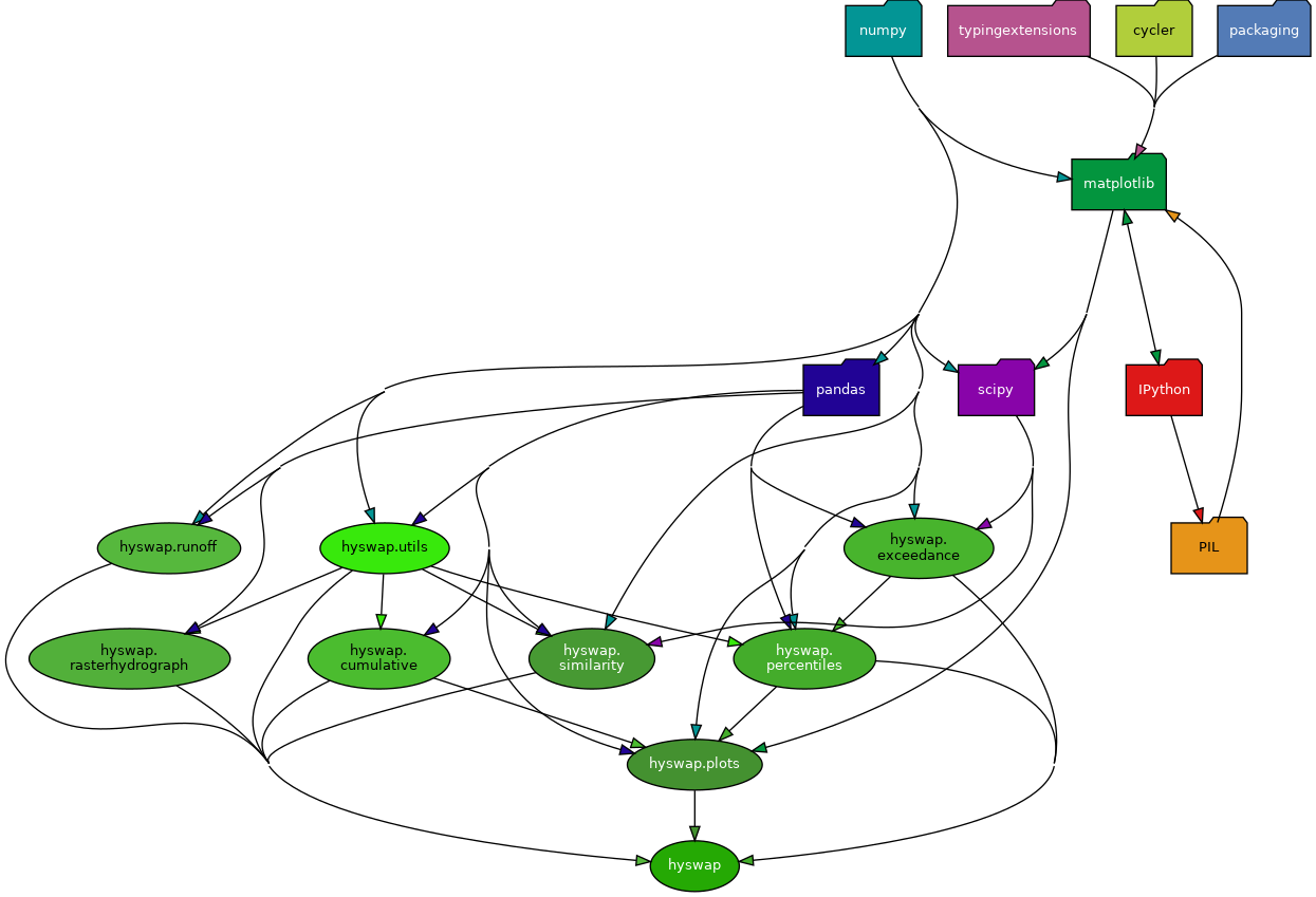
Auto-generated module dependency graph for hyswap as generated by pydeps.

API Reference

Utility Functions

Utility functions for hyswap.

hyswap.utils.calculate_metadata(data)

Calculate metadata for a series of data.

Parameters:

data (pandas.Series) – The data to calculate the metadata for. Expected to have a datetime index.

Returns:

The calculated metadata which includes the number of years of data, the number of data points, any gaps in the data, and the start and end dates of the data, the number of 0 values, the number of NA values, as well as the number of low (typically low flow <= 0.01) values.

Return type:

dict

hyswap.utils.calculate_summary_statistics(df, data_col='00060_Mean')

Calculate summary statistics for a site.

Parameters:

• df (pandas.DataFrame) – DataFrame containing daily values for the site. Expected to be from dataretrieval.nwis.get_dv(), or similar.

• data_col (str, optional) – Name of the column in the dv_df DataFrame that contains the data of interest. Default is “00060_Mean” which is the mean daily discharge column.

Returns:

summary_df – DataFrame containing summary statistics for the site.

Return type:

pandas.DataFrame

Examples

Get some NWIS data and apply the function to get the summary statistics.

>>> df, _ = dataretrieval.nwis.get_dv(
...     "03586500", parameterCd="00060",
...     startDT="2010-01-01", endDT="2010-12-31")
>>> summary_df = utils.calculate_summary_statistics(df)
>>> summary_df.shape
(8, 1)
>>> print(summary_df)
            Summary Statistics
Site number           03586500
Begin date          2010-01-01
End date            2010-12-31
Count                      365
Minimum                   2.48
Mean                    207.43
Median                    82.5
Maximum                 3710.0

hyswap.utils.categorize_flows(df, percentile_col, date_column_name=None, min_years=None, percentile_df=None, schema_name='NWD', custom_schema=None)

Function to categorize streamflows based on percentile ranges

This function assigns a category to each streamflow observation for a single site by comparing the estimated percentile to a schema of percentile ranges and associated category labels

Parameters:

• df (pandas.DataFrame) – DataFrame containing percentile values for date(s) of interest for the site.

• percentile_col (str) – Name of the column in the DataFrame that contains the data of interest, in this case estimated streamflow percentile.

• date_column_name (str, optional) – Name of column containing date information. If None, the index of df is used.

• min_years (int, optional) – Minimum number of years of data required to calculate percentile thresholds for a given day of year. Default is None. Use of min_years setting requires that percentile_df be provided.

• percentile_df (pd.DataFrame) – DataFrame where columns are the percentile thresholds values and the values are stored in a row called “values”. Typically generated by the calculate_fixed_percentile_thresholds or munge_nwis_stats functions but could be provided manually. Must be indexed by month_day and include count column that represents number of years of records for that day of year.

• schema_name (str, optional) – Name of the categorization schema that should be used to categorize streamflow. Default is “NWD” schema.

• custom_schema (dict, optional) – Python dictionary describing custom schema to use for categorizing streamflow based on percentiles. Required in dict is ‘ranges’, an array of percentile cut points and ‘labels’, a list of category labels that matches the number of bins represented by ranges. Optionally can include ‘low_label’ and ‘high_label’ which are category labels associated with the lowest and highest values in ‘ranges’, respectively. Additional optional keys include ‘colors’, ‘low_color’, and ‘high_color’ which specify a color palette that can be accessed in user created plots and maps. Default is None.

Returns:

df – DataFrame with flow_cat column added.

Return type:

pandas.DataFrame

Examples

Categorize streamflow based on calculated percentiles for streamflow records downloaded from NWIS.

>>> data, _ = dataretrieval.nwis.get_dv(
...     "04288000", parameterCd="00060",
...     start="1900-01-01", end="2021-12-31")
>>> pcts_df = percentiles.calculate_variable_percentile_thresholds_by_day(  # noqa: E501
...     data, '00060_Mean',
...     percentiles=[0, 5, 10, 25, 75, 90, 95, 100],
...     method='linear')
>>> new_data, _ = dataretrieval.nwis.get_dv(
...     "04288000", parameterCd="00060",
...     start="2022-05-01", end="2022-05-07")
>>> new_percentiles = percentiles.calculate_multiple_variable_percentiles_from_values(  # noqa: E501
...     new_data, '00060_Mean', pcts_df)
>>> new_percentiles = utils.categorize_flows(new_percentiles,
...     'est_pct', schema_name='NWD')
>>> new_percentiles[['est_pct', 'flow_cat']].values
[[13.62, 'Below normal'],
[14.15, 'Below normal'],
[14.29, 'Below normal'],
[23.41, 'Below normal'],
[27.44, 'Normal'],
[16.2, 'Below normal'],
[12.81, 'Below normal']]

hyswap.utils.define_year_doy_columns(df_in, date_column_name=None, year_type='calendar', clip_leap_day=False)

Function to add year, day of year, and month-day columns to a DataFrame.

Parameters:

• df_in (pandas.DataFrame) – DataFrame containing data to filter. Expects datetime information to be available in the index or in a column named date_column_name.

• date_column_name (str, optional) – Name of column containing date information. If None, the index of df is used.

• year_type (str, optional) – The type of year to use. Must be one of ‘calendar’, ‘water’, or ‘climate’. Default is ‘calendar’ which starts the year on January 1 and ends on December 31. ‘water’ starts the year on October 1 and ends on September 30 of the following year which is the “water year”. For example, October 1, 2010 to September 30, 2011 is “water year 2011”. ‘climate’ years begin on April 1 and end on March 31 of the following year, they are numbered by the ending year. For example, April 1, 2010 to March 31, 2011 is “climate year 2011”.

• clip_leap_day (bool, optional) – If True, February 29 is removed from the DataFrame. Default is False.

Returns:

df – DataFrame with year, day of year, and month-day columns added. Also makes the date_column_name the index of the DataFrame.

Return type:

pandas.DataFrame

hyswap.utils.filter_approved_data(data, filter_column=None)

Filter a dataframe to only return approved “A” (or “A, e”) data.

Parameters:

• data (pandas.DataFrame) – The data to filter.

• filter_column (string) – The column upon which to filter. If None, an error will be raised.

Returns:

The filtered data.

Return type:

pandas.DataFrame

Examples

Filter synthetic data to only return approved data. First make some synthetic data.

>>> df = pd.DataFrame({
...     'data': [1, 2, 3, 4, 5],
...     'approved': ['A', 'A, e', 'A', 'P', 'P']})
>>> df.shape
(5, 2)

Then filter the data to only return approved data.

>>> df = utils.filter_approved_data(df, filter_column='approved')
>>> df.shape
(3, 2)

hyswap.utils.filter_data_by_month_day(df, month_day, data_column_name, date_column_name=None, leading_values=0, trailing_values=0, drop_na=False)

Function used to filter to a single month-day (alternate to filter_data_by_time)

DataFrame containing data to filter. Expects datetime information to be available in the index or in a column named date_column_name. The returned pandas.Series object will have the datetimes for the specified time (day, month, year) as the index, and the corresponding data from the data_column_name column as the values.

Parameters:

• month_day (string) – Time value to use for filtering in the format ‘MM-DD’.

• data_column_name (str) – Name of column containing data to filter.

• date_column_name (str, optional) – Name of column containing date information. If None, the index of df is used.

• leading_values (int, optional) – Number of leading values to include in the output, inclusive. Default is 0, and parameter only applies to ‘day’ time_interval.

• trailing_values (int, optional) – Number of trailing values to include in the output, inclusive. Default is 0, and parameter only applies to ‘day’ time_interval.

• drop_na (bool, optional) – Drop NA values within filtered data

Returns:

data – Data from the specified month-day, plus any leading/trailing values.

Return type:

pandas.Series

Examples

Filter some synthetic data by day of year. First make some synthetic data.

>>> df = pd.DataFrame({
...     'data': [1, 2, 3, 4],
...     'date': pd.date_range('2019-01-01', '2019-01-04')})
>>> df.shape
(4, 2)

Then filter the data to get data from January 1st.

>>> data = utils.filter_data_by_month_day(
...     df, '01-01', 'data', date_column_name='date')
>>> data.shape
(1,)

Acquire and filter some real daily data to get all Jan. 1 data.

>>> df, _ = dataretrieval.nwis.get_dv(
...     "03586500", parameterCd="00060",
...     start="2000-01-01", end="2003-01-05")
>>> data = utils.filter_data_by_month_day(df, '01-01', '00060_Mean')
>>> data.shape
(4,)

hyswap.utils.filter_data_by_time(df, value, data_column_name, date_column_name=None, time_interval='day', leading_values=0, trailing_values=0, drop_na=False)

Filter data by some time interval.

DataFrame containing data to filter. Expects datetime information to be available in the index or in a column named date_column_name. The returned pandas.Series object will have the datetimes for the specified time (day, month, year) as the index, and the corresponding data from the data_column_name column as the values.

Parameters:

• value (int) – Time value to use for filtering; value can be a day of year (1-366), month (1-12), or year (4 digit year).

• data_column_name (str) – Name of column containing data to filter.

• date_column_name (str, optional) – Name of column containing date information. If None, the index of df is used.

• time_interval (str, optional) – Time interval to filter by. Must be one of ‘day’, ‘month’, or ‘year’. Default is ‘day’.

• leading_values (int, optional) – Number of leading values to include in the output, inclusive. Default is 0, and parameter only applies to ‘day’ time_interval.

• trailing_values (int, optional) – Number of trailing values to include in the output, inclusive. Default is 0, and parameter only applies to ‘day’ time_interval.

• drop_na (bool, optional) – Drop NA values within filtered data

Returns:

data – Data from the specified day of year.

Return type:

pandas.Series

Examples

Filter some synthetic data by day of year. First make some synthetic data.

>>> df = pd.DataFrame({
...     'data': [1, 2, 3, 4],
...     'date': pd.date_range('2019-01-01', '2019-01-04')})
>>> df.shape
(4, 2)

Then filter the data to get data from day 1.

>>> data = utils.filter_data_by_time(
...     df, 1, 'data', date_column_name='date')
>>> data.shape
(1,)

Acquire and filter some real daily data to get all Jan. 1 data.

>>> df, _ = dataretrieval.nwis.get_dv(
...     "03586500", parameterCd="00060",
...     start="2000-01-01", end="2003-01-05")
>>> data = utils.filter_data_by_time(df, 1, '00060_Mean')
>>> data.shape
(4,)

hyswap.utils.filter_to_common_time(df_list)

Filter a list of dataframes to common times based on index.

This function takes a list of dataframes and filters them to only include the common times based on the index of the dataframes. This is necessary before comparing the timeseries and calculating statistics between two or more timeseries.

Parameters:

df_list (list) – List of pandas.DataFrame objects to filter to common times. DataFrames assumed to have date-time information in the index. Expect input to be the output from a function like dataretrieval.nwis.get_dv() or similar.

Returns:

• df_list (list) – List of pandas.DataFrame objects filtered to common times.

• n_obs (int) – Number of observations in the common time period.

Examples

Get some NWIS data.

>>> df1, md1 = dataretrieval.nwis.get_dv(
...     "03586500", parameterCd="00060",
...     start="2018-12-15", end="2019-01-07")
>>> df2, md2 = dataretrieval.nwis.get_dv(
...     "01646500", parameterCd="00060",
...     start="2019-01-01", end="2019-01-14")
>>> type(df1)
<class 'pandas.core.frame.DataFrame'>
>>> type(df2)
<class 'pandas.core.frame.DataFrame'>

Filter the dataframes to common times.

>>> df_list, n_obs = utils.filter_to_common_time([df1, df2])
>>> df_list[0].shape
(7, 3)
>>> df_list[1].shape
(7, 3)

hyswap.utils.leap_year_adjustment(df, year_type='calendar')

Function to adjust leap year days in a DataFrame.

Adjust for a leap year by removing February 29 from the DataFrame and adjusting the day of year values for the remaining days of the year if a ‘doy_index’ column is present.

Parameters:

• df (pandas.DataFrame) – DataFrame containing data to adjust. Expects datetime information to be available in the index and a column named ‘doy’ containing day of year.

• year_type (str, optional) – The type of year to use. Must be one of ‘calendar’, ‘water’, or ‘climate’. Default is ‘calendar’ which starts the year on January 1 and ends on December 31. ‘water’ starts the year on October 1 and ends on September 30 of the following year which is the “water year”. For example, October 1, 2010 to September 30, 2011 is “water year 2011”. ‘climate’ years begin on April 1 and end on March 31 of the following year, they are numbered by the ending year. For example, April 1, 2010 to March 31, 2011 is “climate year 2011”. Please note that this input is used to adjust the day of year index when a leap day is removed. If the dataframe does not have a day of year index, this input is ignored.

Returns:

df – DataFrame with leap year days removed and day of year values adjusted.

Return type:

pandas.DataFrame

hyswap.utils.munge_nwis_stats(df, include_metadata=True)

Function to munge and reformat NWIS statistics data.

This is a utility function that exists to help munge NWIS percentile data served via the NWIS statistics web service. This function uses the output of nwis.get_stats() for daily data at a single site and for a single parameter code.

Parameters:

• df (pandas.DataFrame) – DataFrame containing NWIS statistics data retrieved from the statistics web service. Assumed to come in as a dataframe retrieved with a package like dataretrieval or similar.

• include_metadata (bool, optional) – If True, return additional columns from NWIS Stats Service including count, mean, water year of start of record, water year of end of record

Returns:

df – DataFrame containing munged and reformatted NWIS statistics data. Reformatting is to match the format created by calculate_variable_percentile_thresholds_by_day function.

Return type:

pandas.DataFrame

Examples

Get some NWIS statistics data.

>>> df, md = dataretrieval.nwis.get_stats(
...     "03586500", parameterCd="00060", statReportType="daily")

Then apply the function to munge the data.

>>> df = utils.munge_nwis_stats(df)
>>> df.shape
(366, 15)

hyswap.utils.retrieve_schema(schema_name)

Function used to retrieve the flow range categories given a schema name

Parameters:

schema_name (str) – Name of the categorization schema that should be used to categorize streamflow. Available options are ‘NWD’, ‘WaterWatch, ‘WaterWatch_Drought’, ‘WaterWatch_Flood’, ‘WaterWatch_BrownBlue’, and ‘NIDIS_Drought’.

Returns:

schema – dictionary of flow ranges, category labels, and color palette

Return type:

dict

Examples

Retrieve the categorization schema ‘NWD’ to categorization flow similar to the USGS National Water Dashboard

>>> schema = utils.retrieve_schema('NWD')
>>> print(schema)
{'ranges': [0, 10, 25, 76, 90, 100],
'labels': ['Much below normal', 'Below normal', 'Normal',
    'Above normal', 'Much above normal'],
'colors': ['#b24249', '#e8ac49', '#44f24e', '#5fd7d9', '#2641f1'],
'low_label': 'All-time low for this day',
'low_color': '#e82f3e',
'high_label': 'All-time high for this day',
'high_color': '#1f296b'}

hyswap.utils.rolling_average(df, data_column_name, data_type, auto_min_periods=True, custom_min_periods=None, **kwargs)

Calculate a rolling average for a dataframe.

Default behavior right-aligns the window used for the rolling average and uses the data_type argument (‘1D’, ‘7D’, ‘14D’, ‘28D’) to set the min_periods argument in pandas.DataFrame.rolling. The function returns NaN values if any of the values in the window are NaN or if the mind_periods argument is not satisifed. Properties of the windowing can be changed by passing additional keyword arguments which are fed to pandas.DataFrame.rolling.

Parameters:

• df (pandas.DataFrame) – The dataframe to calculate the rolling average for.

• data_column_name (string) – The name of the column to calculate the rolling average for.

• data_type (string) – The formatted frequency string to be used with pandas.DataFrame.rolling to calculate the average over the correct temporal period.

• auto_min_periods (bool) – Defaults to True. When True, the min_periods argument in pandas.DataFrame.rolling is set using the data_type argument. For example, if the data_type = ‘7D’, the min_periods argument is 7. When False, the min_periods argument is set using the custom_min_periods input.

• custom_min_periods (int, optional) – Defaults to None. Only used if auto_min_periods is False. If auto_min_periods is False and an integer is provided, that integer will be used to define the min_periods argument in pandas.DataFrame.rolling.

• **kwargs – Additional keyword arguments to be passed to pandas.DataFrame.rolling.

Returns:

The output dataframe with the rolling average values.

Return type:

pandas.DataFrame

hyswap.utils.set_data_type(data_type)

Function to set the data type for rolling averages.

Parameters:

data_type (str) – The type of data. Must be one of ‘daily’, ‘7-day’, ‘14-day’, and ‘28-day’. If ‘7-day’, ‘14-day’, or ‘28-day’ is specified, the data will be averaged over the specified period. NaN values will be used for any days that do not have data. If present, NaN values will result in NaN values for the entire period.

Returns:

data_type – The formatted frequency string to be used with pandas.DataFrame.rolling to calculate the average over the correct temporal period.

Return type:

str

Exceedance Probability Functions

Exceedance probability calculations.

hyswap.exceedance.calculate_exceedance_probability_from_distribution(x, dist, *args, **kwargs)

Calculate the exceedance probability of a value relative to a distribution.

Parameters:

• x (float) – The value for which to calculate the exceedance probability.

• dist (str) – The distribution to use. Must be one of ‘lognormal’, ‘normal’, ‘weibull’, or ‘exponential’.

• *args – Positional arguments to pass to the distribution, which is one of stats.lognorm.sf, stats.norm.sf, stats.exponweib.sf or stats.expon.sf, refer to the scipy.stats documentation for more information about these arguments.

• **kwargs – Keyword arguments to pass to the distribution, which is one of stats.lognorm.sf, stats.norm.sf, stats.exponweib.sf or stats.expon.sf, refer to the scipy.stats documentation for more information about these arguments.

Returns:

The exceedance probability.

Return type:

float

Examples

Calculating the exceedance probability of a value of 1 from a lognormal distribution with a mean of 1 and a standard deviation of 0.25.

>>> exceedance.calculate_exceedance_probability_from_distribution(
...     1, 'lognormal', 1, 0.25)
0.6132049428659028

Calculating the exceedance probability of a value of 1 from a normal distribution with a mean of 1 and a standard deviation of 0.25.

>>> exceedance.calculate_exceedance_probability_from_distribution(
...     1, 'normal', 1, 0.25)
0.5

hyswap.exceedance.calculate_exceedance_probability_from_distribution_multiple(values, dist, *args, **kwargs)

Calculate the exceedance probability of multiple values vs a distribution.

Parameters:

• values (array-like) – The values for which to calculate the exceedance probability.

• dist (str) – The distribution to use. Must be one of ‘lognormal’, ‘normal’, ‘weibull’, or ‘exponential’.

• *args – Positional arguments to pass to the distribution, which is one of stats.lognorm.sf, stats.norm.sf, stats.exponweib.sf or stats.expon.sf, refer to the scipy.stats documentation for more information about these arguments.

• **kwargs – Keyword arguments to pass to the distribution, which is one of stats.lognorm.sf, stats.norm.sf, stats.exponweib.sf or stats.expon.sf, refer to the scipy.stats documentation for more information about these arguments.

Returns:

The exceedance probabilities.

Return type:

array-like

Examples

Calculating the exceedance probability of a set of values of 1, 1.25 and 1.5 from a lognormal distribution with a mean of 1 and a standard deviation of 0.25.

>>> exceedance.calculate_exceedance_probability_from_distribution_multiple(  # noqa: E501
...     [1, 1.25, 1.5], 'lognormal', 1, 0.25)
array([0.61320494, 0.5       , 0.41171189])

Calculating the exceedance probability of a set of values of 1, 2, 3, and 4 from a normal distribution with a mean of 1 and a standard deviation of 0.25.

>>> exceedance.calculate_exceedance_probability_from_distribution_multiple(  # noqa: E501
...     [1, 2, 3, 4], 'normal', 1, 0.25)
array([5.00000000e-01, 3.16712418e-05, 6.22096057e-16, 1.77648211e-33])

hyswap.exceedance.calculate_exceedance_probability_from_values(x, values_to_compare, method='weibull')

Calculate the exceedance probability of a value compared to several values.

This function computes an exceedance probability using common plotting position formulas, with the default being the ‘Weibull’ method (also known as Type 6 in R). The value (x) is ranked among the values to compare by determining the number that are greater than or equal to the input value (x), which provides the minimum rank in the case of tied values. Additional methods other than the ‘Weibull’ method can be specified and are described in more detail in Helsel et al 2020.

Helsel, D.R., Hirsch, R.M., Ryberg, K.R., Archfield, S.A.,

and Gilroy, E.J., 2020, Statistical methods in water resources: U.S. Geological Survey Techniques and Methods, book 4, chap. A3, 458 p., https://doi.org/10.3133/tm4a3. [Supersedes USGS Techniques of Water-Resources Investigations, book 4, chap. A3, version 1.1.]

Parameters:

• x (float) – The value for which to calculate the exceedance probability.

• values_to_compare (array-like) – The values to use to calculate the exceedance probability.

• method (str, optional) – Method (formulation) of plotting position formula. Default is ‘weibull’ (Type 6). Additional available methods are ‘interpolated_inverted_cdf’ (Type 4), ‘hazen’ (Type 5), ‘linear’ (Type 7), ‘median_unbiased’ (Type 8), and ‘normal_unbiased’ (Type 9).

Returns:

The exceedance probability.

Return type:

float

Examples

Calculating the exceedance probability of a value of 1 from a set of values of 1, 2, 3, and 4.

>>> exceedance.calculate_exceedance_probability_from_values(
...     1, [1, 2, 3, 4], method='linear')
1.0

Calculating the exceedance probability of a value of 5 from a set of values of 1, 2, 3, and 4.

>>> exceedance.calculate_exceedance_probability_from_values(
...     5, [1, 2, 3, 4])
0.0

Fetch some data from NWIS and calculate the exceedance probability for a value of 300 cfs. This is close to the maximum stream flow value for this gage and date range, so the exceedance probability is very small.

>>> df, _ = dataretrieval.nwis.get_dv(
...    site='10171000',
...    start='2000-01-01',
...    end='2020-01-01')
>>> np.round(
...    exceedance.calculate_exceedance_probability_from_values(
...        300, df['00060_Mean']),
...        6)
0.000137

hyswap.exceedance.calculate_exceedance_probability_from_values_multiple(values, values_to_compare, method='weibull')

Calculate the exceedance probability of multiple values vs a set of values. All methods supported in calculate_exceedance_probability_from_values are supported and by default uses the ‘Weibull’ method.

Parameters:

• values (array-like) – The values for which to calculate the exceedance probability.

• values_to_compare (array-like) – The values to use to calculate the exceedance probability.

• method (str, optional) – Method (formulation) of plotting position formula. Default is ‘weibull’ (Type 6). Additional available methods are ‘interpolated_inverted_cdf’ (Type 4), ‘hazen’ (Type 5), ‘linear’ (Type 7), ‘median_unbiased’ (Type 8), and ‘normal_unbiased’ (Type 9).

Returns:

The exceedance probabilities.

Return type:

array-like

Examples

Calculating the exceedance probability of a set of values of 1, 1.25 and 1.5 from a set of values of 1, 2, 3, and 4.

>>> exceedance.calculate_exceedance_probability_from_values_multiple(
...     [1, 1.25, 2.5], [1, 2, 3, 4], method='Type 4')
array([1.  , 0.75, 0.5 ])

Fetch some data from NWIS and calculate the exceedance probability for a set of 5 values spaced evenly between the minimum and maximum values.

>>> df, _ = dataretrieval.nwis.get_gwlevels(site='434400121275801',
...                                         start='2000-01-01',
...                                         end='2020-01-01')
>>> values = np.linspace(df['lev_va'].min(),
...                      df['lev_va'].max(), 5)
>>> exceedance.calculate_exceedance_probability_from_values_multiple(
...     values, df['lev_va'])
array([1.        , 0.96363636, 0.83636364, 0.47272727, 0.01818182])

Raster Hydrograph Functions

Raster hydrograph functionality.

hyswap.rasterhydrograph._calculate_date_range(df, year_type, begin_year, end_year)

Private function to calculate the date range and set the index.

Parameters:

• df (pandas.DataFrame) – The data to format. Must have a date column or the index must be the date values.

• year_type (str) – The type of year to use. Must be one of ‘calendar’, ‘water’, or ‘climate’.

• begin_year (int, None) – The first year to include in the data. If None, the first year in the data will be used.

• end_year (int, None) – The last year to include in the data. If None, the last year in the data will be used.

Returns:

date_range – The date range.

Return type:

pandas.DatetimeIndex

hyswap.rasterhydrograph._check_inputs(df, data_column_name, date_column_name, data_type, year_type, begin_year, end_year, clip_leap_day)

Private function to check inputs for the format_data function.

Parameters:

• df (pandas.DataFrame) – The data to format. Must have a date column or the index must be the date values.

• data_column_name (str) – The name of the column containing the data.

• date_column_name (str, None) – The name of the column containing the date or None if the index is the date.

• data_type (str) – The type of data. Must be one of ‘daily’, ‘7-day’, ‘14-day’, and ‘28-day’. If ‘7-day’, ‘14-day’, or ‘28-day’ is specified, the data will be averaged over the specified period. NaN values will be used for any days that do not have data. If present, NaN values will result in NaN values for the entire period.

• year_type (str) – The type of year to use. Must be one of ‘calendar’ or ‘water’. ‘calendar’ starts the year on January 1 and ends on December 31. ‘water’ starts the year on October 1 and ends on September 30.

• begin_year (int, None) – The first year to include in the data. If None, the first year in the data will be used.

• end_year (int, None) – The last year to include in the data. If None, the last year in the data will be used.

• clip_leap_day (bool, optional) – If True, removes leap day ‘02-29’ from the percentiles dataset used to create the plot.

Returns:

df – The dataframe with the date column formatted as a datetime and set as the index. New year and doy (day of year) columns are added too and are set based on the year_type. Feb 29th is also removed from the dataframe if it exists.

Return type:

pandas.DataFrame

hyswap.rasterhydrograph.format_data(df, data_column_name, date_column_name=None, data_type='daily', year_type='calendar', begin_year=None, end_year=None, clip_leap_day=False, **kwargs)

Format data for raster hydrograph.

Parameters:

• df (pandas.DataFrame) – The data to format. Must have a date column or the index must be the date values.

• data_column_name (str) – The name of the column containing the data.

• date_column_name (str, optional) – The name of the column containing the date. Default is None which assumes the index is the date.

• data_type (str, optional) – The type of data. Must be one of ‘daily’, ‘7-day’, ‘14-day’, and ‘28-day’. Default is ‘daily’. If ‘7-day’, ‘14-day’, or ‘28-day’ is specified, the data will be averaged over the specified period. NaN values will be used for any days that do not have data. If present, NaN values will result in NaN values for the entire period.

• year_type (str, optional) – The type of year to use. Must be one of ‘calendar’, ‘water’, or ‘climate’. Default is ‘calendar’ which starts the year on January 1 and ends on December 31. ‘water’ starts the year on October 1 and ends on September 30 of the following year which is the “water year”. For example, October 1, 2010 to September 30, 2011 is “water year 2011”. ‘climate’ years begin on April 1 and end on March 31 of the following year, they are numbered by the ending year. For example, April 1, 2010 to March 31, 2011 is “climate year 2011”.

• begin_year (int, optional) – The first year to include in the data. Default is None which uses the first year in the data.

• end_year (int, optional) – The last year to include in the data. Default is None which uses the last year in the data.

• clip_leap_day (bool, optional) – If True, removes leap day ‘02-29’ from the percentiles dataset used to create the plot. Defaults to False.

• **kwargs – Keyword arguments to pass to the pandas.DataFrame.rolling method.

Returns:

The formatted data starting on the first day of the first year and ending on the last day of the last year with the specified data type and year type.

Return type:

pandas.DataFrame

Examples

Formatting synthetic daily data for a raster hydrograph.

>>> df = pd.DataFrame({'date': pd.date_range('1/1/2010', '12/31/2010'),
...                    'data': np.random.rand(365)})
>>> df_formatted = rasterhydrograph.format_data(df, 'data', 'date')
>>> df_formatted.index[0]
2010
>>> len(df_formatted.columns)
365

Formatting real daily data for a raster hydrograph.

>>> df, _ = dataretrieval.nwis.get_dv(
...     "03586500", parameterCd="00060",
...     start="2000-01-01", end="2002-12-31")
>>> df_formatted = rasterhydrograph.format_data(df, '00060_Mean')
>>> df_formatted.index[0]
2000
>>> len(df_formatted.columns)
365

Percentile Calculation Functions

Percentile calculation functions.

hyswap.percentiles.calculate_fixed_percentile_from_value(value, percentile_df)

Calculate percentile from a value and fixed percentile thresholds.

This function enables faster calculation of the percentile associated with a given value if percentile values and corresponding fixed percentile thresholds are known from other data from the same station or site. This calculation is done using linear interpolation. A value greater than the largest streamflow value in the percentile threshold dataframe results in a percentile of 100. A value less than the smallest streamflow value in the percentile threshold dataframe results in a percentile of 0.

Parameters:

• value (float, np.ndarray) – New value(s) to calculate percentile for. Can be a single value or an array of values.

• percentile_df (pd.DataFrame) – DataFrame where columns are the percentile thresholds values and the values are stored in a row called “values”. Typically generated by the calculate_fixed_percentile_thresholds functions but could be provided manually or from data pulled from the NWIS stats service.

Returns:

percentile – Percentile associated with the input value(s).

Return type:

float, np.ndarray

Examples

Calculate the percentile associated with a value from some synthetic data.

>>> data = pd.DataFrame({'values': np.arange(1001),
...                      'date': pd.date_range('2020-01-01', '2022-09-27')}).set_index('date')  # noqa: E501
>>> pcts_df = percentiles.calculate_fixed_percentile_thresholds(
...     data, 'values', percentiles=[5, 10, 25, 50, 75, 90, 95])
>>> new_percentile = percentiles.calculate_fixed_percentile_from_value(
...     500, pcts_df)
>>> new_percentile
50.0

Calculate the percentiles associated with multiple values for some data downloaded from NWIS.

>>> data, _ = dataretrieval.nwis.get_dv(
...     "04288000", parameterCd="00060",
...     start="1900-01-01", end="2021-12-31")
>>> pcts_df = percentiles.calculate_fixed_percentile_thresholds(
...     data, '00060_Mean',
...     percentiles=[5, 10, 25, 50, 75, 90, 95,],
...     method='linear')
>>> new_data, _ = dataretrieval.nwis.get_dv(
...     "04288000", parameterCd="00060",
...     start="2022-01-01", end="2022-01-07")
>>> new_data['est_pct'] = percentiles.calculate_fixed_percentile_from_value(  # noqa: E501
...     new_data['00060_Mean'], pcts_df)
>>> new_data['est_pct'].to_list()
[62.9, 75.0, 55.65, 47.54, 53.55, 55.32, 50.97]

hyswap.percentiles.calculate_fixed_percentile_thresholds(data, data_column_name=None, percentiles=array([5, 10, 25, 50, 75, 90, 95]), method='weibull', date_column_name=None, ignore_na=True, include_min_max=True, include_metadata=True, mask_out_of_range=True, **kwargs)

Calculate fixed percentile thresholds using historical data.

Parameters:

• data (pandas.DataFrame or array-like) – DataFrame, Series, or 1-D array containing data used to calculate percentile thresholds. If DataFrame, “data_column_name” must be specified and expects a datetime index unless “date_column_name” is provided. If Series, must include a datetime index. If 1-D array, then “include_metadata” must be set to False since a datetime index is not included with data.

• data_column_name (str, optional) – Name of column containing data to analyze if input is a DataFrame. Default is None.

• percentiles (array_like, optional) – Percentiles to calculate. Default is (5, 10, 25, 50, 75, 90, 95). Note: Values of 0 and 100 are ignored as unbiased plotting position formulas do not assign values to 0 or 100th percentile.

• method (str, optional) – Method to use to calculate percentiles. Default is ‘weibull’ (Type 6). Additional available methods are ‘interpolated_inverted_cdf’ (Type 4), ‘hazen’ (Type 5), ‘linear’ (Type 7), ‘median_unbiased’ (Type 8), and ‘normal_unbiased’ (Type 9).

• date_column_name (str, optional) – For data provided as DataFrame, name of column containing date information. If None, the index of data is used.

• ignore_na (bool, optional) – Ignore NA values in percentile calculations

• include_min_max (bool, optional) – When set to True, include min and max streamflow value in addition to streamflow values for percentile levels. Default is True.

• include_metadata (bool, optional) – When set to True, return additional columns describing the data including count, mean, start_yr, end_yr. Default is True. Input data must include a datetime column as either index or specified by date_column_name.

• mask_out_of_range (bool, optional) – When set to True, percentiles that are beyond the min/max percentile ranks of the observed data to be NA. Effect of this being enables is that high or low percentiles may not be calculated when few data points are available. Default is True.

• **kwargs (dict, optional) – Additional keyword arguments to pass to numpy.percentile.

Returns:

percentiles – Percentiles of the data in a DataFrame so the thresholds and percentile values are tied together.

Return type:

pandas.DataFrame

Examples

Calculate percentile thresholds from some synthetic data using ‘linear’ method.

>>> data = pd.DataFrame({'values': np.arange(101),
...                      'date': pd.date_range('2020-01-01', '2020-04-10')}).set_index('date')  # noqa: E501
>>> results = percentiles.calculate_fixed_percentile_thresholds(
...     data, 'values', percentiles=[25, 75, 95], method='linear')
>>> results
        min   p25   p75   p95  max  mean  count start_yr end_yr
values    0  25.0  75.0  95.0  100  50.0    101     2020   2020

Calculate percentile thresholds without additional metadata columns

>>> data = np.arange(101)
>>> results = percentiles.calculate_fixed_percentile_thresholds(
...     data, percentiles=[5, 25, 75, 95], method='linear',
...     include_metadata=False)
>>> results
        min  p05   p25   p75   p95  max
values    0  5.0  25.0  75.0  95.0  100

Calculate percentile thresholds using default ‘weibull’ method

>>> data = np.arange(101)
>>> results = percentiles.calculate_fixed_percentile_thresholds(
...     data, percentiles=[5, 25, 50, 75, 95],
...     include_metadata=False)
>>> results
        min  p05   p25   p50   p75   p95  max
values    0  4.1  24.5  50.0  75.5  95.9  100

Calculate percentile thresholds from a small number of observations and mask out out of range percentile levels

>>> data = np.arange(11)
>>> results = percentiles.calculate_fixed_percentile_thresholds(
...     data, percentiles=np.array((1, 10, 50, 90, 99)),
...     include_metadata=False)
>>> results
        min  p01  p10  p50  p90  p99  max
values    0  NaN  0.2  5.0  9.8  NaN   10

hyswap.percentiles.calculate_multiple_variable_percentiles_from_values(df, data_column_name, percentile_df, date_column_name=None)

Calculate variable percentiles for multiple values

This function enables calculation of estimated percentiles for multiple values across multiple days of the year using existing variable percentile thresholds. This calculation is done using linear interpolation. A value greater than the largest streamflow value in the percentile threshold dataframe for the month-day of interest results in a percentile of 100. A value less than the smallest streamflow value in the percentile threshold dataframe results in a percentile of 0.

Parameters:

• df (pd.DataFrame) – Pandas dataframe containing new values to calculate percentiles for.

• data_column_name (str) – Name of column containing data to analyze.

• percentile_df (pd.DataFrame) – DataFrame containing threshold percentiles of data by day of year. Typically generated by the calculate_variable_percentile_thresholds functions but could be provided manually or from data pulled from the NWIS stats service.

• date_column_name (str, optional) – Name of column containing date information. If None, the index of df is used.

Returns:

df – Pandas dataframe of values with estimated percentile column added

Return type:

pd.DataFrame

Examples

Calculate the percentiles associated with multiple values using flow records downloaded from NWIS.

>>> data, _ = dataretrieval.nwis.get_dv(
...     "04288000", parameterCd="00060",
...     start="1900-01-01", end="2021-12-31")
>>> pcts_df = percentiles.calculate_variable_percentile_thresholds_by_day(  # noqa: E501
...     data, '00060_Mean',
...     percentiles=[5, 10, 25, 50, 75, 90, 95],
...     method='linear')
>>> new_data, _ = dataretrieval.nwis.get_dv(
...     "04288000", parameterCd="00060",
...     start="2022-01-01", end="2022-01-07")
>>> new_percentiles = percentiles.calculate_multiple_variable_percentiles_from_values(  # noqa: E501
...     new_data, '00060_Mean', pcts_df)
>>> new_percentiles['est_pct'].to_list()
[64.81, 77.7, 56.67, 45.0, 55.59, 59.38, 49.12]

hyswap.percentiles.calculate_variable_percentile_from_value(value, percentile_df, month_day)

Calculate percentile from a value and variable percentile thresholds.

This function enables faster calculation of the percentile associated with a given value for a single day of the year if percentile values and corresponding variable percentile thresholds are known from other data from the same station or site. This calculation is done using linear interpolation. A value greater than the largest streamflow value in the percentile threshold dataframe for the month-day of interest results in a percentile of 100. A value less than the smallest streamflow value in the percentile threshold dataframe results in a percentile of 0.

Parameters:

• value (float, np.ndarray) – New value(s) to calculate percentile for. Can be a single value or an array of values.

• percentile_df (pd.DataFrame) – DataFrame containing threshold percentiles of data by day of year. Typically generated by the calculate_variable_percentile_thresholds function but could be provided manually or from data pulled from the NWIS stats service.

• month_day (str) – string of month-day of year to lookup percentile thresholds for value

Returns:

percentile – Percentile associated with the input value(s).

Return type:

float, np.ndarray

Examples

Calculate the percentile associated with a value using flow records downloaded from NWIS.

>>> data, _ = dataretrieval.nwis.get_dv(
...     "03586500", parameterCd="00060",
...     start="1776-01-01", end="2022-12-31")
>>> pcts_df = percentiles.calculate_variable_percentile_thresholds_by_day(  # noqa: E501
...     data, '00060_Mean',
...     percentiles=[5, 10, 25, 50, 75, 90, 95],
...     method='linear')
>>> new_percentile = percentiles.calculate_variable_percentile_from_value(  # noqa: E501
...     500, pcts_df, '06-30')
>>> new_percentile
96.58

hyswap.percentiles.calculate_variable_percentile_thresholds_by_day(df, data_column_name, percentiles=[5, 10, 25, 50, 75, 90, 95], method='weibull', date_column_name=None, data_type='daily', leading_values=0, trailing_values=0, clip_leap_day=False, ignore_na=True, include_min_max=True, include_metadata=True, mask_out_of_range=True, **kwargs)

Calculate variable percentile thresholds of data by day

Parameters:

• df (pandas.DataFrame) – DataFrame containing data to calculate daily percentile thresholds for.

• data_column_name (str) – Name of column containing data to analyze.

• percentiles (array_like, optional) – Percentile thresholds to calculate, default is [5, 10, 25, 50, 75, 90, 95]. Note: Values of 0 and 100 are ignored as unbiased plotting position formulas do not assign values to 0 or 100th percentile.

• method (str, optional) – Method to use to calculate percentiles. Default is ‘weibull’ (Type 6). Additional available methods are ‘interpolated_inverted_cdf’ (Type 4), ‘hazen’ (Type 5), ‘linear’ (Type 7), ‘median_unbiased’ (Type 8), and ‘normal_unbiased’ (Type 9).

• date_column_name (str, optional) – Name of column containing date information. If None, the index of df is used.

• data_type (str, optional) – The type of data. Must be one of ‘daily’, ‘7-day’, ‘14-day’, and ‘28-day’. Default is ‘daily’. If ‘7-day’, ‘14-day’, or ‘28-day’ is specified, the data will be averaged over the specified period. NaN values will be used for any days that do not have data. If present, NaN values will result in NaN values for the entire period.

• leading_values (int, optional) – For the temporal filtering, this is an argument setting the number of leading values to include in the output, inclusive. Default is 0, and parameter only applies to ‘day’ time_interval.

• trailing_values (int, optional) – For the temporal filtering, this is an argument setting the number of trailing values to include in the output, inclusive. Default is 0, and parameter only applies to ‘day’ time_interval.

• clip_leap_day (bool, optional) – If True, February 29 is removed from the DataFrame. Default is False.

• ignore_na (bool, optional) – Ignore NA values in percentile calculations

• include_min_max (bool, optional) – When set to True, include min and max streamflow value in addition to streamflow values for percentile levels. Default is True.

• include_metadata (bool, optional) – When set to True, return additional columns describing the data including count, mean, start_yr, end_yr. Default is True

• mask_out_of_range (bool, optional) – When set to True, percentiles that are beyond the min/max percentile ranks of the observed data to be NA. Effect of this being enables is that high or low percentiles may not be calculated when few data points are available. Default is True.

• **kwargs (dict, optional) – Additional keyword arguments to pass to numpy.percentile.

Returns:

percentiles – DataFrame containing threshold percentiles of data by month-day. Will return a DataFrame of NaNs for each percentile/day if provided an empty DataFrame or DataFrame with insufficient data

Return type:

pandas.DataFrame

Examples

Calculate default thresholds by day from some real data in preparation for plotting.

>>> df, _ = dataretrieval.nwis.get_dv(
...     "03586500", parameterCd="00060",
...     start="1776-01-01", end="2022-12-31")
>>> results = percentiles.calculate_variable_percentile_thresholds_by_day(  # noqa: E501
...     df, "00060_Mean")
>>> len(results.index)  # 366 days in a leap year
366

hyswap.percentiles.calculate_variable_percentile_thresholds_by_day_of_year(df, data_column_name, percentiles=[5, 10, 25, 50, 75, 90, 95], method='weibull', date_column_name=None, data_type='daily', year_type='calendar', leading_values=0, trailing_values=0, clip_leap_day=False, ignore_na=True, include_min_max=True, include_metadata=True, mask_out_of_range=True, **kwargs)

Calculate variable percentile thresholds of data by day of year.

Parameters:

• df (pandas.DataFrame) – DataFrame containing data to calculate daily percentile thresholds for.

• data_column_name (str) – Name of column containing data to analyze.

• percentiles (array_like, optional) – Percentile thresholds to calculate, default is [5, 10, 25, 50, 75, 90, 95]. Note: Values of 0 and 100 are ignored as unbiased plotting position formulas do not assign values to 0 or 100th percentile.

• method (str, optional) – Method to use to calculate percentiles. Default is ‘weibull’ (Type 6). Additional available methods are ‘interpolated_inverted_cdf’ (Type 4), ‘hazen’ (Type 5), ‘linear’ (Type 7), ‘median_unbiased’ (Type 8), and ‘normal_unbiased’ (Type 9).

• date_column_name (str, optional) – Name of column containing date information. If None, the index of df is used.

• data_type (str, optional) – The type of data. Must be one of ‘daily’, ‘7-day’, ‘14-day’, and ‘28-day’. Default is ‘daily’. If ‘7-day’, ‘14-day’, or ‘28-day’ is specified, the data will be averaged over the specified period. NaN values will be used for any days that do not have data. If present, NaN values will result in NaN values for the entire period.

• year_type (str, optional) – The type of year to use. Must be one of ‘calendar’, ‘water’, or ‘climate’. Default is ‘calendar’ which starts the year on January 1 and ends on December 31. ‘water’ starts the year on October 1 and ends on September 30 of the following year which is the “water year”. For example, October 1, 2010 to September 30, 2011 is “water year 2011”. ‘climate’ years begin on April 1 and end on March 31 of the following year, they are numbered by the ending year. For example, April 1, 2010 to March 31, 2011 is “climate year 2011”.

• leading_values (int, optional) – For the temporal filtering, this is an argument setting the number of leading values to include in the output, inclusive. Default is 0, and parameter only applies to ‘day’ time_interval.

• trailing_values (int, optional) – For the temporal filtering, this is an argument setting the number of trailing values to include in the output, inclusive. Default is 0, and parameter only applies to ‘day’ time_interval.

• clip_leap_day (bool, optional) – If True, February 29 is removed from the DataFrame. Default is False.

• ignore_na (bool, optional) – Ignore NA values in percentile calculations

• include_min_max (bool, optional) – When set to True, include min and max streamflow value in addition to streamflow values for percentile levels. Default is True.

• include_metadata (bool, optional) – When set to True, return additional columns describing the data including count, mean, start_yr, end_yr. Default is True

• mask_out_of_range (bool, optional) – When set to True, percentiles that are beyond the min/max percentile ranks of the observed data to be NA. Effect of this being enables is that high or low percentiles may not be calculated when few data points are available. Default is True.

• **kwargs (dict, optional) – Additional keyword arguments to pass to numpy.percentile.

Returns:

percentiles – DataFrame containing threshold percentiles of data by day of year. The DataFrame has a multi-index of ‘doy’ and ‘year_type’. Returns a DataFrame of NaNs for each percentile/day if provided an empty DataFrame or DataFrame with insufficient data

Return type:

pandas.DataFrame

Examples

Calculate default thresholds by day of year from some real data in preparation for plotting.

>>> df, _ = dataretrieval.nwis.get_dv(
...     "03586500", parameterCd="00060",
...     start="1776-01-01", end="2022-12-31")
>>> results = percentiles.calculate_variable_percentile_thresholds_by_day_of_year(  # noqa: E501
...     df, "00060_Mean")
>>> len(results.index)  # 366 days in a leap year
366

Cumulative Calculation Functions

Cumulative calculation functions.

hyswap.cumulative._tidy_cumulative_dataframe(cdf, year_type)

Tidy a cumulative dataframe.

Parameters:

• cdf (pandas.DataFrame) – DataFrame containing cumulative values, rows are years, columns are days of year.

• year_type (str) – The type of year to use. Must be one of ‘calendar’, ‘water’, or ‘climate’. Default is ‘calendar’ which starts the year on January 1 and ends on December 31. ‘water’ starts the year on October 1 and ends on September 30 of the following year which is the “water year”. For example, October 1, 2010 to September 30, 2011 is “water year 2011”. ‘climate’ years begin on April 1 and end on March 31 of the following year, they are numbered by the ending year. For example, April 1, 2010 to March 31, 2011 is “climate year 2011”.

Returns:

cdf – DataFrame containing cumulative values, rows are dates, columns include years, day of year (doy), and cumulative values.

Return type:

pandas.DataFrame

hyswap.cumulative.calculate_daily_cumulative_values(df, data_column_name, date_column_name=None, year_type='calendar', unit='acre-feet', clip_leap_day=False)

Calculate daily cumulative values.

Parameters:

• df (pandas.DataFrame) – DataFrame containing data to calculate cumulative values.

• data_column_name (str) – Name of column containing data to calculate cumulative values for. Discharge data assumed to be in unit of ft3/s.

• date_column_name (str, optional) – Name of column containing date information. If None, the index of df will be used.

• year_type (str, optional) – The type of year to use. Must be one of ‘calendar’, ‘water’, or ‘climate’. Default is ‘calendar’ which starts the year on January 1 and ends on December 31. ‘water’ starts the year on October 1 and ends on September 30 of the following year which is the “water year”. For example, October 1, 2010 to September 30, 2011 is “water year 2011”. ‘climate’ years begin on April 1 and end on March 31 of the following year, they are numbered by the ending year. For example, April 1, 2010 to March 31, 2011 is “climate year 2011”.

• unit (str, optional) – The unit the user wants to use to report cumulative flow. One of ‘acre-feet’, ‘cfs’, ‘cubic-meters’, ‘cubic-feet’. Assumes input data are in cubic feet per second (cfs).

Returns:

cumulative_values – DataFrame containing daily cumulative values for each year in the input DataFrame, rows are dates and columns include years, month-days, day-of-year and cumulative values in the units specified.

Return type:

pandas.DataFrame

Examples

Calculate daily cumulative values from some synthetic data.

>>> df = pd.DataFrame({
...     "date": pd.date_range("2000-01-01", "2000-12-31"),
...     "data": np.arange(366)})
>>> results = cumulative.calculate_daily_cumulative_values(
...     df, "data", date_column_name="date")
>>> results.columns.tolist()
['index_month_day', 'index_year', 'index_doy', 'cumulative']

Plotting Functions

Functions for plotting.

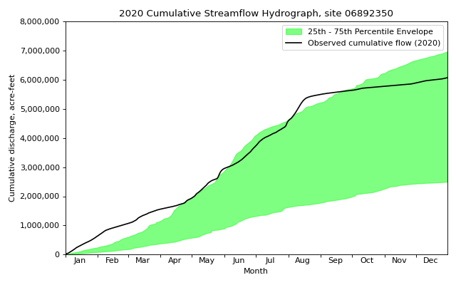
hyswap.plots.plot_cumulative_hydrograph(df, target_years, data_column_name, date_column_name=None, year_type='calendar', unit='acre-feet', envelope_pct=[25, 75], max_year=False, min_year=False, ax=None, disclaimer=False, title='Cumulative Streamflow Hydrograph', ylab='Cumulative discharge, acre-feet', xlab='Month', clip_leap_day=False, **kwargs)

Plot a cumulative hydrograph.

The cumulative-streamflow hydrograph is a graphical presentation of recent cumulative daily streamflow (discharge) observed at an individual USGS streamgage, plotted over the long-term statistics of streamflow for each day of the year at that station. Typically, the statistics, based on quality assured and approved data, include the maximum annual cumulative discharge recorded during the period of record; the mean-daily cumulative flow for each day; the minimum cumulative discharge recorded for each day.

Note: For some streams, flow statistics may have been computed from mixed regulated and unregulated flows; this can affect depictions of flow conditions.

Parameters:

• df (pandas.DataFrame) – Dataframe containing the data to plot.

• target_years (int, or list) – Target year(s) to plot in black as the line. Can provide a single year as an integer, or a list of years.

• data_column_name (str) – Name of column containing data to calculate cumulative values for. Discharge data assumed to be in unit of ft3/s.

• date_column_name (str, optional) – Name of column containing date information. If None, the index of df will be used.

• unit (str, optional) – The unit the user wants to use to report cumulative flow. One of ‘acre-feet’, ‘cfs’, ‘cubic-meters’, ‘cubic-feet’. Assumes input data are in cubic feet per second (cfs).

• envelope_pct (list, optional) – List of percentiles to plot as the envelope. Default is [25, 75]. If an empty list, [], then no envelope is plotted.

• max_year (bool, optional) – If True, plot the cumulative flow for the year with the maximum end of the year cumulative value as a dashed line. Default is False.

• min_year (bool, optional) – If True, plot the cumulative flow for the year with the minimum end of the year cumulative value as a dashed line. Default is False.

• ax (matplotlib.axes.Axes, optional) – Axes to plot on. If not provided, a new figure and axes will be created.

• disclaimer (bool, optional) – If True, displays the disclaimer ‘For some streams, flow statistics may have been computed from mixed regulated and unregulated flows; this can affect depictions of flow conditions.’ below the x-axis.

• title (str, optional) – Title for the plot. If not provided, the default title will be ‘Cumulative Streamflow Hydrograph’.

• ylab (str, optional) – Label for the y-axis. If not provided, the default label will be ‘Cumulative Streamflow, ft3/s’.

• xlab (str, optional) – Label for the x-axis. If not provided, the default label will be ‘Month’.

• clip_leap_day (bool, optional) – If True, removes leap day ‘02-29’ from the percentiles dataset used to create the plot. Defaults to False.

• **kwargs – Keyword arguments passed to matplotlib.axes.Axes.fill_between().

Returns:

Axes object containing the plot.

Return type:

matplotlib.axes.Axes

Examples

Fetch some data from NWIS and make a cumulative hydrograph plot.

>>> df, _ = dataretrieval.nwis.get_dv(site='06892350',
...                                   parameterCd='00060',
...                                   start='1900-01-01',
...                                   end='2021-12-31')
>>> fig, ax = plt.subplots(figsize=(8, 5))
>>> ax = hyswap.plots.plot_cumulative_hydrograph(
...     df,
...     data_column_name='00060_Mean',
...     target_years=2020, ax=ax,
...     title='2020 Cumulative Streamflow Hydrograph, site 06892350')
>>> plt.tight_layout()
>>> plt.show()

(png, hires.png)

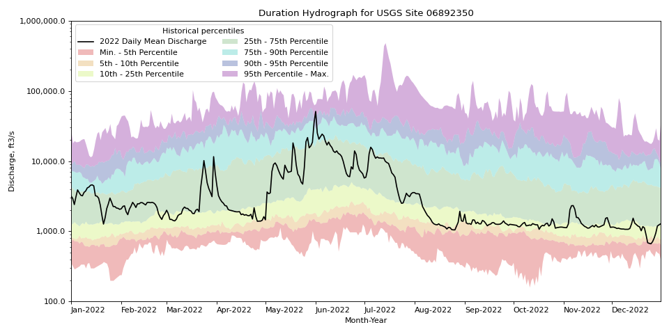
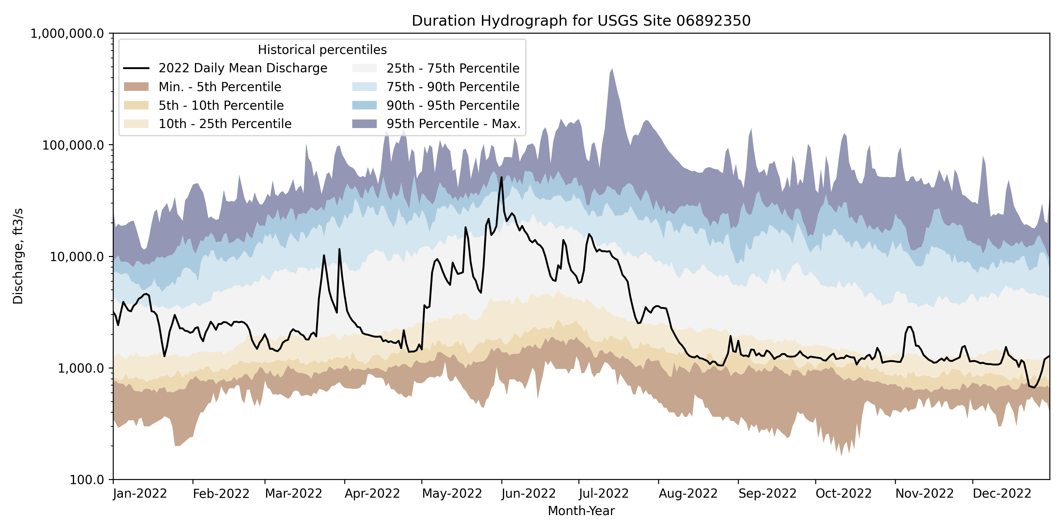
hyswap.plots.plot_duration_hydrograph(percentiles_by_day, df, data_col, date_column_name=None, pct_list=[5, 10, 25, 75, 90, 95], data_label=None, ax=None, disclaimer=False, title='Duration Hydrograph', ylab='Discharge, ft3/s', xlab='Month-Year', colors=None, **kwargs)

Plot a duration hydrograph.

The duration hydrograph is a graphical presentation of recent daily streamflow (discharge) observed at an individual USGS streamgage, plotted over the long-term statistics of streamflow for each day of the year at that station. Typically, the statistics (based on quality assured and approved data) include the maximum discharge recorded during the period of record for each day of the year; the 90th percentile flow for each day; the interquartile range (75th percentile on top and 25th percentile on the bottom); the 10th percentile flow for each day; and the minimum discharge recorded for each day. This function, however, allows the user to plot a custom list of percentiles.

Note: For some streams, flow statistics may have been computed from mixed regulated and unregulated flows; this can affect depictions of flow conditions.

Parameters:

• percentiles_by_day (pandas.DataFrame) – Dataframe containing the percentiles by month-day. Note that this plotting function is incompatible with percentiles calculated by day-of-year.

• df (pandas.DataFrame) – Dataframe containing the data to plot.

• data_col (str) – Column name of the data to plot.

• date_column_name (str, optional) – Defaults to None. If None, index is assumed to contain datetime information.

• pct_list (list, optional) – List of integers corresponding to the percentile values to be plotted. Values of 0 and 100 are ignored as unbiased plotting position formulas do not assign values to 0 or 100th percentile. Defaults to 5, 10, 25, 75, 90, 95.

• data_label (str, optional) – Label for the data to plot. If not provided, a default label will be used.

• ax (matplotlib.axes.Axes, optional) – Axes to plot on. If not provided, a new figure and axes will be created.

• disclaimer (bool, optional) – If True, displays the disclaimer ‘For some streams, flow statistics may have been computed from mixed regulated and unregulated flows; this can affect depictions of flow conditions.’ below the x-axis.

• title (str, optional) – Title for the plot. If not provided, the default title will be ‘Duration Hydrograph’.

• ylab (str, optional) – Label for the y-axis. If not provided, the default label will be ‘Discharge, ft3/s’.

• xlab (str, optional) – Label for the x-axis. If not provided, the default label will be ‘Month’.

• colors (list, optional) – List of colors to use for the lines. If not provided, a default list of colors will be used. The max number of colors in this list is seven.

• **kwargs – Keyword arguments passed to matplotlib.axes.Axes.fill_between().

Returns:

Axes object containing the plot.

Return type:

matplotlib.axes.Axes

Examples

Fetch some data from NWIS and make a streamflow duration hydrograph plot.

>>> df, _ = dataretrieval.nwis.get_dv(site='06892350',
...                                   parameterCd='00060',
...                                   start='1900-01-01',
...                                   end='2022-12-31')
>>> pct_by_day = hyswap.percentiles.calculate_variable_percentile_thresholds_by_day(  # noqa: E501
...     df, '00060_Mean')
>>> df_2022 = df[df.index.year == 2022]
>>> fig, ax = plt.subplots(figsize=(12, 6))
>>> ax = hyswap.plots.plot_duration_hydrograph(
...     pct_by_day, df_2022, '00060_Mean',
...     data_label='2022 Daily Mean Discharge',
...     ax=ax, title='Duration Hydrograph for USGS Site 06892350')
>>> plt.tight_layout()
>>> plt.show()

(png, hires.png)

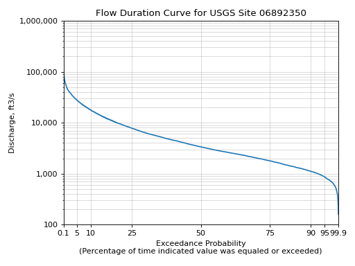
hyswap.plots.plot_flow_duration_curve(values, exceedance_probabilities, observations=None, observation_probabilities=None, ax=None, title='Flow Duration Curve', xlab='Exceedance Probability\n(Percentage of time indicated value was equaled or exceeded)', ylab='Discharge, ft3/s', grid=True, scatter_kwargs={}, **kwargs)

Plot a flow duration curve.

Flow duration curves are cumulative frequency curves that show the percentage of time measured discharge values are equaled or exceeded by all other discharge values in the dataset.

Parameters:

• values (array-like) – Values to plot along y-axis.

• exceedance_probabilities (array-like) – Exceedance probabilities for each value, likely calculated from a function like hyswap.exceedance.calculate_exceedance_probability_from_values_multiple.

• observations (list, numpy.ndarray, optional) – List, numpy array or list-able set of flow observations. Optional, if not provided the observations are not plotted.

• observation_probabilities (list, numpy.ndarray, optional) – Exceedance probabilities corresponding to each observation, likely calculated from a function like hyswap.exceedance.calculate_exceedance_probability_from_values_multiple. Optional, if not provided observations are not plotted.

• ax (matplotlib.axes.Axes, optional) – Axes to plot on. If not provided, a new figure and axes will be created.

• title (str, optional) – Title for the plot. If not provided, the default title will be ‘Flow Duration Curve’.

• xlab (str, optional) – Label for the x-axis. If not provided, a default label will be used.

• ylab (str, optional) – Label for the y-axis. If not provided, a default label will be used.

• grid (bool, optional) – Whether to show grid lines on the plot. Default is True.

• scatter_kwargs (dict) – Dictionary containing keyword arguments to pass to the observations plotting method, matplotlib.axes.Axes.scatter().

• **kwargs – Keyword arguments passed to matplotlib.axes.Axes.plot().

Returns:

Axes object containing the plot.

Return type:

matplotlib.axes.Axes

Examples

Fetch some data from NWIS, calculate the exceedance probabilities and then make the flow duration curve.

>>> df, _ = dataretrieval.nwis.get_dv(site='06892350',
...                                   parameterCd='00060',
...                                   start='1776-07-04',
...                                   end='2020-01-01')
>>> values = np.linspace(df['00060_Mean'].min(),
...                      df['00060_Mean'].max(), 10000)
>>> exceedance_probabilities = hyswap.exceedance.calculate_exceedance_probability_from_values_multiple(  # noqa
...     values, df['00060_Mean'])
>>> ax = hyswap.plots.plot_flow_duration_curve(
...     values, exceedance_probabilities,
...     title='Flow Duration Curve for USGS Site 06892350')
>>> plt.tight_layout()
>>> plt.show()

(png, hires.png)

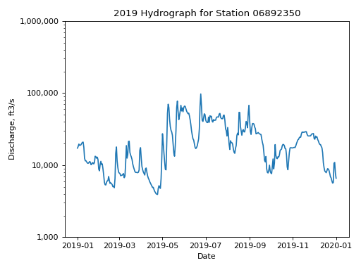
hyswap.plots.plot_hydrograph(df, data_col, date_col=None, start_date=None, end_date=None, ax=None, title='Streamflow Hydrograph', ylab='Discharge, ft3/s', xlab='Date', yscale='log', **kwargs)

Plot a simple hydrograph.

Hydrographs show the streamflow discharge over time at a single station.

Parameters:

• df (pandas.DataFrame) – DataFrame containing the data to plot.

• data_col (str) – Name of the column containing the data to plot.

• date_col (str, optional) – Name of the column containing the dates. If not provided, the index will be used.

• start_date (str, optional) – Start date for the plot. If not provided, the minimum date in the DataFrame will be used.

• end_date (str, optional) – End date for the plot. If not provided, the maximum date in the DataFrame will be used.

• ax (matplotlib.axes.Axes, optional) – Axes object to plot on. If not provided, a new figure and axes will be created.

• title (str, optional) – Title of the plot. Default is ‘Streamflow Hydrograph’.

• ylab (str, optional) – Y-axis label. Default is ‘Streamflow, ft3/s’.

• xlab (str, optional) – X-axis label. Default is ‘Date’.

• yscale (str, optional) – Y-axis scale. Default is ‘log’. Options are ‘linear’ or ‘log’.

• **kwargs – Additional keyword arguments to pass to matplotlib.pyplot.plot().

Returns:

Axes object containing the plot.

Return type:

matplotlib.axes.Axes

Examples

Fetch data for a USGS gage and plot the hydrograph.

>>> siteno = '06892350'
>>> df, _ = dataretrieval.nwis.get_dv(site=siteno,
...                                   parameterCd='00060',
...                                   start='2019-01-01',
...                                   end='2020-01-01')
>>> ax = hyswap.plots.plot_hydrograph(
...     df, data_col='00060_Mean',
...     title=f'2019 Hydrograph for Station {siteno}',
...     ylab='Discharge, ft3/s',
...     xlab='Date', yscale='log')
>>> plt.tight_layout()
>>> plt.show()

(png, hires.png)

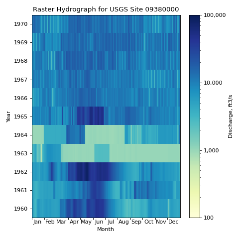
hyswap.plots.plot_raster_hydrograph(df_formatted, ax=None, title='Raster Hydrograph', xlab='Month', ylab='Year', cbarlab='Discharge, ft3/s', **kwargs)

Plot a raster hydrograph.

Raster hydrographs are pixel-based plots for visualizing and identifying variations and changes in large multidimensional data sets. Originally developed by Keim (2000), they were first applied in hydrology by Koehler (2004) as a means of highlighting inter-annual and intra-annual changes in streamflow. The raster hydrographs in hyswap, like those developed by Koehler, depict years on the y-axis and days along the x-axis. Users can choose to plot streamflow (actual values or log values), streamflow percentile, or streamflow class (from 1, for low flow, to 7 for high flow), for Daily, 7-Day, 14-Day, and 28-Day streamflow. For a more comprehensive description of raster hydrographs, see Strandhagen et al. (2006).

References: Keim, D.A. 2000. Designing pixel-oriented visualization techniques: theory and applications. IEEE Transactions on Visualization and Computer Graphics, 6(1), 59-78.

Koehler, R. 2004. Raster Based Analysis and Visualization of Hydrologic Time Series. Ph.D dissertation, University of Arizona. Tucson, AZ, 189 p.

`Strandhagen, E., Marcus, W.A., and Meacham, J.E. 2006. Views of the rivers: representing streamflow of the greater Yellowstone ecosystem. Cartographic Perspectives, no. 55, 54-29.`__

Parameters:

• df_formatted (pandas.DataFrame) – Formatted dataframe containing the raster hydrograph data.

• ax (matplotlib.axes.Axes, optional) – Axes to plot on. If not provided, a new figure and axes will be created.

• title (str, optional) – Title for the plot. If not provided, the default title will be ‘Streamflow Raster Hydrograph’.

• xlab (str, optional) – Label for the x-axis. If not provided, the default label will be ‘Month’.

• ylab (str, optional) – Label for the y-axis. If not provided, the default label will be ‘Year’.

• cbarlab (str, optional) – Label for the colorbar. If not provided, the default label will be ‘Discharge, ft3/s’.

• **kwargs – Keyword arguments passed to matplotlib.axes.Axes.imshow().

Returns:

Axes object containing the plot.

Return type:

matplotlib.axes.Axes

Examples

Fetch some data from NWIS, format it for a raster hydrograph plot and then make the raster hydrograph plot.

>>> df, _ = dataretrieval.nwis.get_dv(site='09380000',
...                                   parameterCd='00060',
...                                   start='1960-01-01',
...                                   end='1970-12-31')
>>> df_rh = hyswap.rasterhydrograph.format_data(df, '00060_Mean')
>>> fig, ax = plt.subplots(figsize=(6, 6))
>>> ax = hyswap.plots.plot_raster_hydrograph(
...     df_rh, ax=ax, title='Raster Hydrograph for USGS Site 09380000')
>>> plt.tight_layout()
>>> plt.show()

(png, hires.png)

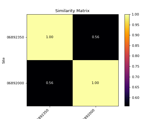
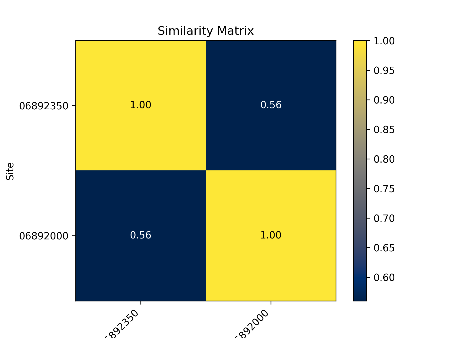
hyswap.plots.plot_similarity_heatmap(sim_matrix, n_obs=None, cmap='inferno', show_values=False, ax=None, title='Similarity Matrix')

Plot a similarity matrix heatmap.

The heatmap shows the results of a correlation matrix between measurements at two or more sites. Lighter, warmer colors denote higher similarity (correlation), while darker colors denote less similarity between two sites.

Parameters:

• sim_matrix (pandas.DataFrame) – Similarity matrix to plot. Must be square. Can be the output of hyswap.similarity.calculate_correlations(), hyswap.similarity.calculate_wasserstein_distance(), hyswap.similarity.calculate_energy_distance(), or any other square matrix represented as a pandas DataFrame.

• cmap (str, optional) – Colormap to use. Default is ‘inferno’.

• show_values (bool, optional) – Whether to show the values of the matrix on the plot. Default is False.

• ax (matplotlib.axes.Axes, optional) – Axes object to plot on. If not provided, a new figure and axes will be created.

• title (str, optional) – Title for the plot. Default is ‘Similarity Matrix’.

Returns:

Axes object containing the plot.

Return type:

matplotlib.axes.Axes

Examples

Calculate the correlation matrix between two sites and plot it as a heatmap.

>>> df, _ = dataretrieval.nwis.get_dv(site='06892350',
...                                   parameterCd='00060',
...                                   start='2010-01-01',
...                                   end='2021-12-31')
>>> df2, _ = dataretrieval.nwis.get_dv(site='06892000',
...                                    parameterCd='00060',
...                                    start='2010-01-01',
...                                    end='2021-12-31')
>>> corr_matrix, n_obs = hyswap.similarity.calculate_correlations(
...     [df, df2], '00060_Mean')
>>> ax = hyswap.plots.plot_similarity_heatmap(corr_matrix,
...                                           show_values=True)
>>> plt.show()

(png, hires.png)

Runoff Calculation Functions

Runoff functions for hyswap.

hyswap.runoff._get_date_range(df_list, start_date, end_date)

Get date range for runoff calculation.

This is an internal function used by the calculate_geometric_runoff function to get the date range for the runoff calculation. If no start or end date is specified, the earliest/latest date in the df_list will be used.

Parameters:

• df_list (list) – List of dataframes containing runoff data for each site in the geometry.

• start_date (str, optional) – Start date for the runoff calculation. If not specified, the earliest date in the df_list will be used. Format is ‘YYYY-MM-DD’.

• end_date (str, optional) – End date for the runoff calculation. If not specified, the latest date in the df_list will be used. Format is ‘YYYY-MM-DD’.

Returns:

DatetimeIndex containing the date range for the runoff calculation.

Return type:

pandas.DatetimeIndex

hyswap.runoff.calculate_geometric_runoff(geom_id, runoff_dict, geom_intersection_df, site_col, geom_id_col, prop_geom_in_basin_col='prop_huc_in_basin', prop_basin_in_geom_col='prop_basin_in_huc', percentage=False, clip_downstream_basins=True, full_overlap_threshold=0.98)

Function to calculate the runoff for a specified geometry. Uses tabular dataframe containing proportion of geometry in each intersecting basin and proportion of intersecting basins in the specified geometry, as well as a dictionary of basin runoff values.

Parameters:

• geom_id (str) – Geometry ID for the geometry of interest.

• runoff_dict (dict) – Dictionary of dataframes containing runoff data for each site in the geometry. Dictionary key is expected to be the name of the gage site. Each dictionary item is expected to have a date index entitled ‘datetime’ and a data column entitled ‘runoff’ filled with runoff data.

• geom_intersection_df (pandas.DataFrame) – Tabular dataFrame containing columns indicating the site numbers, geometry ids, proportion of geometry in basin, and proportion of basin within geometry.

• site_col (str) – Column in geom_intersection_df with drainage area site numbers. Please make sure ids have the correct number of digits and have not lost leading 0s when read in. If the site numbers are the geom_intersection_df index col, site_col = ‘index’.

• geom_id_col (str) – Column in geom_intersection_df with geometry ids.

• prop_geom_in_basin_col (str) – Name of column with values (type:float) representing the proportion (0 to 1) of the spatial geometry occurring in the corresponding drainage area. Default name: ‘prop_in_basin’

• prop_basin_in_geom_col (str) – Name of column with values (type:float) representing the proportion (0 to 1) of the drainage area occurring in the corresponding spatial geometry. Default name: ‘prop_in_huc’

• percentage (boolean, optional) – If the values in geom_intersection_df are percentages, percentage = True. If the values are decimal proportions, percentage = False. Default: False

• clip_downstream_basins (boolean, optional) – When True, the function estimates runoff using only basins that are (a) contained within the geometry and (b) the smallest basin containing the geometry in the weighted average. When False, the function uses all overlapping basins to estimate runoff for the geometry. Defaults to True.

• full_overlap_threshold (float, optional) – The minimum proportion of overlap between geometry and basin that constitutes “full” overlap. For example, occasionally a geometry (or basin) may be completely contained by a basin (or geometry), but polygon border artifacts might cause the intersection to be slightly less than 1. This input accounts for that error. Defaults to 0.98.

Returns:

Series containing the area-weighted runoff values for the geometry.

Return type:

pandas.Series

hyswap.runoff.calculate_multiple_geometric_runoff(geom_id_list, runoff_dict, geom_intersection_df, site_col, geom_id_col, prop_geom_in_basin_col='prop_huc_in_basin', prop_basin_in_geom_col='prop_basin_in_huc', percentage=False, clip_downstream_basins=True, full_overlap_threshold=0.98)

Calculate runoff for multiple geometries at once.

Parameters:

• geom_id_list (list) – List of geometry ID strings for the geometries of interest. These should be columns in the weights matrix.

• runoff_dict (dict) – Dictionary of dataframes containing runoff data for each site in the geometry. Dictionary key is expected to be the name of the gage site. Each dictionary entry is expected to have a date index and a data column filled with runoff data.

• geom_intersection_df (pandas.DataFrame) – Tabular dataFrame containing columns indicating the site numbers, geometry ids, proportion of geometry in basin, and proportion of basin within geometry.

• site_col (str) – Column in geom_intersection_df with drainage area site numbers. Please make sure ids have the correct number of digits and have not lost leading 0s when read in. If the site numbers are the geom_intersection_df index col, site_col = ‘index’.

• geom_id_col (str) – Column in geom_intersection_df with geometry ids.

• prop_geom_in_basin_col (str) – Name of column with values (type:float) representing the proportion (0 to 1) of the spatial geometry occurring in the corresponding drainage area. Default name: ‘pct_in_basin’

• prop_basin_in_geom_col (str) – Name of column with values (type:float) representing the proportion (0 to 1) of the drainage area occurring in the corresponding spatial geometry. Default name: ‘pct_in_huc’

• percentage (boolean, optional) – If the values in geom_intersection_df are percentages, percentage = True. If the values are decimal proportions, percentage = False. Default: False

• clip_downstream_basins (boolean, optional) – When True, the function estimates runoff using only basins that are (a) contained within the geometry and (b) the smallest basin containing the geometry in the weighted average. When False, the function uses all overlapping basins to estimate runoff for the geometry. Defaults to True.

• full_overlap_threshold (float, optional) – The minimum proportion of overlap between geometry and basin that constitutes “full” overlap. For example, occasionally a geometry (or basin) may be completely contained by a basin (or geometry), but polygon border artifacts might cause the intersection to be slightly less than 1. This input accounts for that error. Defaults to 0.98.

Returns:

DataFrame containing the area-weighted runoff values for each geometry. Columns are geometry IDs, index is date range.

Return type:

pandas.DataFrame

hyswap.runoff.convert_cfs_to_runoff(cfs, drainage_area, frequency='annual')

Convert cfs to runoff values for some drainage area.

Parameters:

• cfs (float) – Flow in cubic feet per second.

• drainage_area (float) – Drainage area in km2.

• frequency (str, optional) – Frequency of runoff values to return. Options are ‘annual’, ‘monthly’, and ‘daily’. Default is ‘annual’.

Returns:

Runoff in mm/<frequency>.

Return type:

float

Examples

Convert 14 cfs to mm/yr for a 250 km2 drainage area.

>>> mmyr = runoff.convert_cfs_to_runoff(14, 250)
>>> np.round(mmyr)
50.0

hyswap.runoff.identify_sites_from_geom_intersection(geom_id, geom_intersection_df, geom_id_col, site_col, prop_geom_in_basin_col='prop_huc_in_basin', prop_basin_in_geom_col='prop_basin_in_huc')

Identify sites for a specified geometry.

Function to identify streamgage sites that have drainage areas intersecting a given spatial geometry (e.g. HUC8) from the output table of a previously computed spatial intersection of drainage areas and spatial geometries. This function is a helper function that can be used to reduce the number of NWIS queries that are performed to construct the list of dataframes for a given geometry.

Parameters:

• geom_id (str) – Geometry ids to filter to (e.g. geom_id = ‘03030006’). Ids range from 8 to 10 digits and sometime involve a leading 0.

• geom_intersection_df (pandas.DataFrame) – Tabular dataFrame containing columns indicating the site numbers, geometry ids, proportion of geometry in basin, and proportion of basin within geometry.

• geom_id_col (str) – Column in geom_intersection_df with geometry ids.

• site_col (str) – Column in geom_intersection_df with drainage area site numbers. Please make sure ids have the correct number of digits and have not lost leading 0s when read in. If the site numbers are the geom_intersection_df index col, site_col = ‘index’.

• prop_geom_in_basin_col (str, optional) – Name of column with values (type:float) representing the proportion (0 to 1) of the spatial geometry occurring in the corresponding drainage area. Default name: ‘prop_huc_in_basin’

• prop_basin_in_geom_col (str, optional) – Name of column with values (type:float) representing the proportion (0 to 1)of the drainage area occurring in the corresponding spatial geometry. Default name: ‘prop_basin_in_huc’

Returns:

List of site IDs with drainage areas that intersect the geometry

Return type:

list

Examples

Find all drainage area site numbers that intersect with geometry id 0101002

>>> data = [['01014000', '01010002', 0.01, 0.6],
...     ['01014001', '01010002', 0.2, 0.8],
...     ['01014002', '01010003', 0.9, 0.05]]
>>> df = pd.DataFrame(data,
... columns = ['site_no', 'geom_id', 'prop_huc_in_basin',
... 'prop_basin_in_huc'])
>>> sites_lst = runoff.identify_sites_from_geom_intersection(
... geom_intersection_df=df, geom_id='01010002',
... geom_id_col='geom_id', site_col='site_no',
... prop_geom_in_basin_col='prop_huc_in_basin',
... prop_basin_in_geom_col='prop_basin_in_huc')
>>> print(sites_lst)
['01014000', '01014001']

hyswap.runoff.streamflow_to_runoff(df, data_col, drainage_area, frequency='annual')

Convert streamflow to runoff for a given drainage area.

For a given gage/dataframe, convert streamflow to runoff using the drainage area and the convert_cfs_to_runoff function.

Parameters:

• df (pandas.DataFrame) – DataFrame containing streamflow data.

• data_col (str) – Column name containing streamflow data, assumed to be in cfs.

• drainage_area (float) – Drainage area in km2.

• frequency (str, optional) – Frequency of runoff values to return. Options are ‘annual’, ‘monthly’, and ‘daily’. Default is ‘annual’.

Returns:

DataFrame containing runoff data in a column named ‘runoff’.

Return type:

pandas.DataFrame

Examples

Convert streamflow to runoff for a given drainage area.

>>> df = pd.DataFrame({'streamflow': [14, 15, 16]})
>>> runoff_df = runoff.streamflow_to_runoff(df, 'streamflow', 250)
>>> print(runoff_df['runoff'].round(1))
0    50.0
1    53.6
2    57.2
Name: runoff, dtype: float64

Similarity Functions

Similarity measures for hyswap.

hyswap.similarity._name_handling(df_list, df_names)

Private function to handle the names of the dataframes.

hyswap.similarity.calculate_correlations(df_list, data_column_name, df_names=None)

Calculate Pearson correlations between dataframes in df_list.

This function is designed to calculate the Pearson correlation coefficients between dataframes in df_list. The dataframes in df_list are expected to have the same columns. The correlation coefficients are calculated using the numpy.corrcoeff function.

Parameters:

• df_list (list) – List of dataframes. The dataframes are expected to have the same columns. Likely inputs are the output of a function like dataretrieval.nwis.get_dv() or similar

• data_column_name (str) – Name of the column to use for the correlation calculation.

• df_names (list, optional) – List of names for the dataframes in df_list. If provided, the names will be used to label the rows and columns of the output array. If not provided, the column “site_no” will be used if available, if it is not available, the index of the dataframe in the list will be used.

Returns:

• correlations (pandas.DataFrame) – Dataframe of correlation coefficients. The rows and columns are labeled with the names of the dataframes in df_list as provided by df_names argument.

• n_obs (int) – Number of observations used to calculate the energy distance.

Examples

Calculate correlations between two synthetic dataframes.

>>> df1 = pd.DataFrame({'a': np.arange(10), 'b': np.arange(10)})
>>> df2 = pd.DataFrame({'a': -1*np.arange(10), 'b': np.arange(10)})
>>> results, n_obs = similarity.calculate_correlations([df1, df2], 'a')
>>> results
     0    1
0  1.0 -1.0
1 -1.0  1.0

hyswap.similarity.calculate_energy_distance(df_list, data_column_name, df_names=None)

Calculate energy distance between dataframes in df_list.

This function is designed to calculate the energy distance between dataframes in df_list. The dataframes in df_list are expected to have the same columns. The energy distance is calculated using the scipy.stats.energy_distance function.

Parameters:

• df_list (list) – List of dataframes. The dataframes are expected to have the same columns. Likely inputs are the output of a function like dataretrieval.nwis.get_dv() or similar

• data_column_name (str) – Name of the column to use for the energy distance calculation.

• df_names (list, optional) – List of names for the dataframes in df_list. If provided, the names will be used to label the rows and columns of the output array. If not provided, the column “site_no” will be used if available, if it is not available, the index of the dataframe in the list will be used.

Returns:

• energy_distances (pandas.DataFrame) – Dataframe of energy distances. The rows and columns are labeled with the names of the dataframes in df_list as provided by df_names argument.

• n_obs (int) – Number of observations used to calculate the energy distance.

Examples

Calculate energy distances between two synthetic dataframes.

>>> df1 = pd.DataFrame({'a': np.arange(10), 'b': np.arange(10)})
>>> df2 = pd.DataFrame({'a': -1*np.arange(10), 'b': np.arange(10)})
>>> results, n_obs = similarity.calculate_energy_distance(
...     [df1, df2], 'a')
>>> results
          0         1
0  0.000000  3.376389
1  3.376389  0.000000

hyswap.similarity.calculate_wasserstein_distance(df_list, data_column_name, df_names=None)

Calculate Wasserstein distance between dataframes in df_list.

This function is designed to calculate the Wasserstein distance between dataframes in df_list. The dataframes in df_list are expected to have the same columns. The Wasserstein distance is calculated using the scipy.stats.wasserstein_distance function.

Parameters:

• df_list (list) – List of dataframes. The dataframes are expected to have the same columns. Likely inputs are the output of a function like dataretrieval.nwis.get_dv() or similar

• data_column_name (str) – Name of the column to use for the Wasserstein distance calculation.

• df_names (list, optional) – List of names for the dataframes in df_list. If provided, the names will be used to label the rows and columns of the output array. If not provided, the column “site_no” will be used if available, if it is not available, the index of the dataframe in the list will be used.

Returns:

• wasserstein_distances (pandas.DataFrame) – Dataframe of Wasserstein distances. The rows and columns are labeled with the names of the dataframes in df_list as provided by df_names argument.

• n_obs (int) – Number of observations used to calculate the energy distance.

Examples

Calculate Wasserstein distances between two synthetic dataframes.

>>> df1 = pd.DataFrame({'a': np.arange(10), 'b': np.arange(10)})
>>> df2 = pd.DataFrame({'a': -1*np.arange(10), 'b': np.arange(10)})
>>> results, n_obs = similarity.calculate_wasserstein_distance(
...     [df1, df2], 'a')
>>> results
     0    1
0  0.0  9.0
1  9.0  0.0