Using SFRmaker with a configuration file

For many applications, the easiest way to get started with SFRmaker is to create a configuration file that can then be used in a simple script to generate an SFR package. The two example problems below illustrate the use of SFRmaker with a configuration file. A comprehensive summary of configuration file inputs is provided in the reference section.

MERAS 3: Creating an SFR package from a configuration file with custom hydrography

This example illustrates the use of custom hydrography with the configuration file, as well the scalability of SFRmaker. An SFR package is generated on a regular 1 km grid (Clark and others, 2018) that spans the Mississippi Embayment, a former bay of the Gulf of Mexico that includes portions of Missouri, Tennessee, Arkansas, Mississippi and Louisiana. The goal is to update the stream network for the Mississippi Embayment Regional Aquifer System (MERAS 2) model (Haugh and others, 2020; Clark and others, 2013) to include a realistic representation of the thousands of mapped streams (Figure 1). NHDPlus hydrography were preprocessed to only include the lines intersecting the MERAS footprint that had a total upstream drainage (arbolate sum) of 20 kilometers or greater (figure 1). Attribute information from NHDPlus, including routing connections, elevations at the upstream and downstream ends of line arcs and channel widths estimated from arbolate sum values (e.g. ref: Feinstein and others (2010, p 266)) were joined to the culled flowlines, which were then saved to a shapefile.

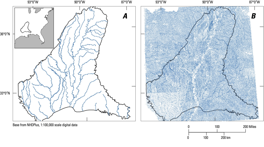
Figure 1: Location of the MERAS model domain with streams represented in the MERAS 2 model (A); streams mapped in NHDPlus version 2 (B).

Many streams enter the Mississippi Embayment with appreciable flow, which must be accounted for in the SFR package to achieve a realistic mass balance. Inflows to the SFR network for this study were derived from a combination of streamgage records and estimates from a statistical model (ref: MS water res. conference abstract). Inflow values for each site and model stress period were saved in a comma-separated-variable (CSV) format.

The configuration file for the Mississippi Embayment example is shown below. The configuration file, associate python script, and input files needed to reproduce the example are available on the SFRmaker GitHub page. The configuration file is specified in the YAML format, which maps key: value pairs similar to a Python dictionary. In the SFRmaker configuration file, keys (to the left of the colons) indicate variables or groups of variables; values to apply to those variables are listed to the right of the colons.

meras_sfrmaker_config.yml:

package_version: 'mf6'
package_name: 'meras3'
output_path: 'meras3'
modelgrid:
  xoffset: 177955
  yoffset: 938285
  nrow: 666
  ncol: 634
  delr: 1000  # model spacing along a row
  delc: 1000  # model spacing along a column
  crs: 5070  # albers equal area
flowlines:
  filename: flowlines.shp
  id_column: COMID  # arguments to sfrmaker.Lines.from_shapefile
  routing_column: tocomid
  width1_column: width1
  width2_column: width2
  up_elevation_column: elevupsmo
  dn_elevation_column: elevdnsmo
  name_column: GNIS_NAME
  attr_length_units: feet  # units of source data
  attr_height_units: feet  # units of source data
inflows:  # see sfrmaker.flows.add_to_perioddata for arguments
  filename: inflows.csv
  line_id_column: line_id
  period_column: per  # column with model stress periods
  data_column: inflow_m3d  # column with flow values
observations:  # see sfrmaker.observations.add_observations for arguments
  filename: observations.csv
  obstype: downstream-flow  # modflow-6 observation type
  x_location_column: x  # observation locations, in CRS coordinates
  y_location_column: y
  obsname_column: site_no  # column for naming observations
options:
  active_area: MERAS_Extent.shp
  one_reach_per_cell: True #  consolidate SFR reaches to one per i, j location
  # add breaks in routing at the following line ids
  # (flow downstream is controlled by dams, and specified as an inflow)
  add_outlets: [18019782, 15276792, 15290344, 15256386]

Information on the model grid is specified in the modelgrid: block of the configuration file. The xoffset and yoffset arguments are the location of the lower left corner of the model grid, in units of the CRS defined by the EPSG code (typically meters). Since this is a uniform grid, only scalar values are provided for the row and column spacing. Variable row and column spacings can be specified using the list notation in YAML, or more simply by loading a flopy model instance into a Python script. SFRmaker does not require a modflow model as input, but a model can be optionally be specified in the configuration file with the model: and simulation: blocks (the latter is only needed for MODFLOW-6 models).

An advantage of specifying a model is that sfmaker will automatically assign stream reaches to the correct layer, based on the layer top and bottom elevations, and account for inactive cells. If the model has correct georeference information in the namefile header as assigned by FloPy, the modelgrid: block is not needed. An optional active_area: allows geographic area for generation of the SFR package input (that may or may not coincide with the active area of the model) to be defined. Otherwise, SFR input will be generated for the extent of the model grid.

While the MERAS hydrography includes elevations, this may not always be the case, or more accurate elevations may be available from a digital elevation model (DEM). If a dem: block is specified and set_streambed_top_elevations_from_dem: True, SFRmaker will sample the DEM to the stream reaches as described in the methods section. The default buffer distance is 100 in the units of the projected CRS, or another buffer distance can be specified with an optional buffer_distance: argument.

The inflows: block allows for specification inflows to the SFR network. Inflow time series must include model stress period information (SFRmaker does not do any resampling) and column names in the input csv file must be specified. Similarly, an observations: block allows observation site locations to be specified in the coordinates of the projected CRS specified for the model grid, or using identifiers corresponding to flowlines in the input hydrography. With this information information, SFRmaker will generate input to the Gage Package (e.g. Prudic, 2004) or Modflow-6 observation utility (Langevin and others, 2017).

The options: block can include keyword arguments to sfrmaker.lines.Lines.to_sfr(), or other options such as set_streambed_top_elevations_from_dem:.

The above configuration file can be used to generate an SFR package with the following Python code:

make_sfr.py:

"""Run the MERAS example.
"""
import sfrmaker
sfrdata = sfrmaker.SFRData.from_yaml('meras_sfrmaker_config.yml')

This will produce an sfr package for MODFLOW-6, csv table representations of the SFR input, and shapefiles for visualizing the SFR package. The resulting SFR package is shown in Figure 2.

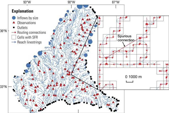
Figure 2: MERAS 3 SFR package, as shown by the shapefiles output from SFRmaker. Visualization of routing connections is illustrated in the map inset, where a connection crossing several cells indicates an error in the input hydrography routing attributes.

The Tyler Forks watershed: Creating an SFR package from a configuration file using NHDPlus

This example shows how a configuration file can be used to build an SFR package from NHDPlus data, with a model grid specified using a MODFLOW model or a shapefile. The example is set in the Tyler Forks watershed in northern Wisconsin, where groundwater/surface interactions are the primary modeling interest.

In the first configuration file, the Name file and workspace for a MODFLOW-NWT model are specified. An active area denoting where the SFR package will be built is provided with a shapefile. NHDPlus data are provided as a file path to the root folder level for a drainage basin (for example, 04, The Great Lakes), assuming the files within that path are in the same structure as the download from the NHDPlus website. Finally, a dem is provided as a a more accurate source of streambed elevations.

tf_sfrmaker_config.yml:

model:
  namefile: tf.nam
  model_ws: tylerforks/
flowlines:
  nhdplus_paths: NHDPlus/
dem:
  filename: dem_26715.tif
  elevation_units: meters
options:
  active_area: active_area.shp

In the second configuration file, no model is specified, so a package version, name, output path and length units are specified. The model grid is specified from a shapefile that has attribute fields indicating the row, column location of each cell. NHPlus data a specified as individual files.

package_version: 'mfnwt'
package_name: 'tf'
output_path: '.'
modelgrid:
  shapefile: grid.shp
  icol: i  # attribute field with row numbers
  jcol: j  # attribute field with column numbers
flowlines:
  NHDFlowlines: NHDPlus/NHDSnapshot/Hydrography/NHDFlowline.shp
  PlusFlowlineVAA: NHDPlus/NHDPlusAttributes/PlusFlowlineVAA.dbf
  PlusFlow: NHDPlus/NHDPlusAttributes/PlusFlow.dbf
  elevslope: NHDPlus/NHDPlusAttributes/elevslope.dbf
inflows: # see sfrmaker.flows.add_to_segment_data for arguments
  filename: inflows.csv
  line_id_column: line_id_COMID
  period_column: SP  # column with model stress periods
  data_column: inflow_m3d  # column with flow values
dem:
  filename: dem_26715.tif
  elevation_units: meters
  buffer_distance: 50.
options:
  model_length_units: 'feet'

Either of these configuration files can then be used with a python script similar to the following:

tylerforks/make_sfr.py:

"""Run the Tyler Forks example.
"""
import sfrmaker
sfrdata = sfrmaker.SFRData.from_yaml('tf_sfrmaker_config.yml')

This will produce an sfr package for MODFLOW-NWT, csv table representations of the SFR input, and shapefiles for visualizing the SFR package.

Running the tylerforks model

The above script can be found in the examples/tylerforks folder of the SFRmaker repository. Assuming the script was run from that location, the resulting MODFLOW model can then be run using the MODFLOW executable packaged with SFRmaker (on Windows):

cd tylerforks
../../../bin/win/mfnwt.exe tf.nam

(or on OSX)

cd tylerforks
../../../bin/mac/mfnwt tf.nam