Plotting with nhdplusTools
The goal of this vignette is to demonstrate a simple and lightweight approach to building maps with NHDPlus data.
The plot_nhdplus function
plot_nhdplus is a work in progress. Not all
inputs in the function have been implemented as of 11/18/2019 and
additional functionality will be added later. Please leave feature
requests and issues you find in an issue
here.
plot_nhdplus is a function that makes getting a simple
plot of NHDPlus data as easy as possible. It works with other functions
from nhdplusTools for identifying and retrieving watershed
outlet locations. See the plot_nhdplus documentation for
more info.
If we pass plot_nhdplus a single NWIS site id,
nhdplusTools uses web services to get data and we get a
plot like this:
plot_nhdplus("05428500")
If we want to add other watersheds, we can use any outlet available
from the Network Linked Data Index. See “nldi” functions elsewhere in
nhdplusTools.
plot_nhdplus(list(list("nwissite", "USGS-05428500"),
                  list("huc12pp", "070900020602")))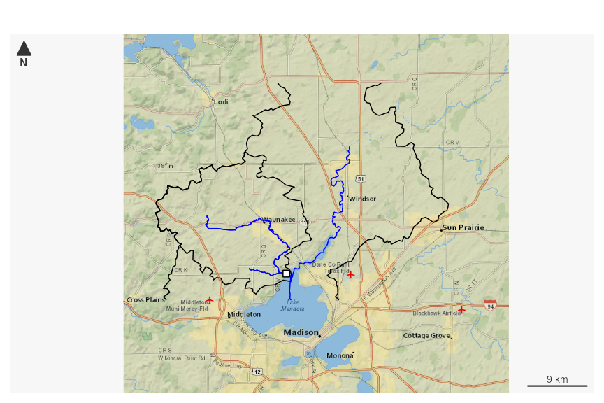
plot_nhdplus(list(list("nwissite", "USGS-05428500"),
                  list("huc12pp", "070900020602")))
If we don’t know a site id, we can just pass in one or more latitude / longitude locations.
start_point <- sf::st_as_sf(data.frame(x = -89.36, y = 43.09),
                            coords = c("x", "y"), crs = 4326)

plot_nhdplus(start_point)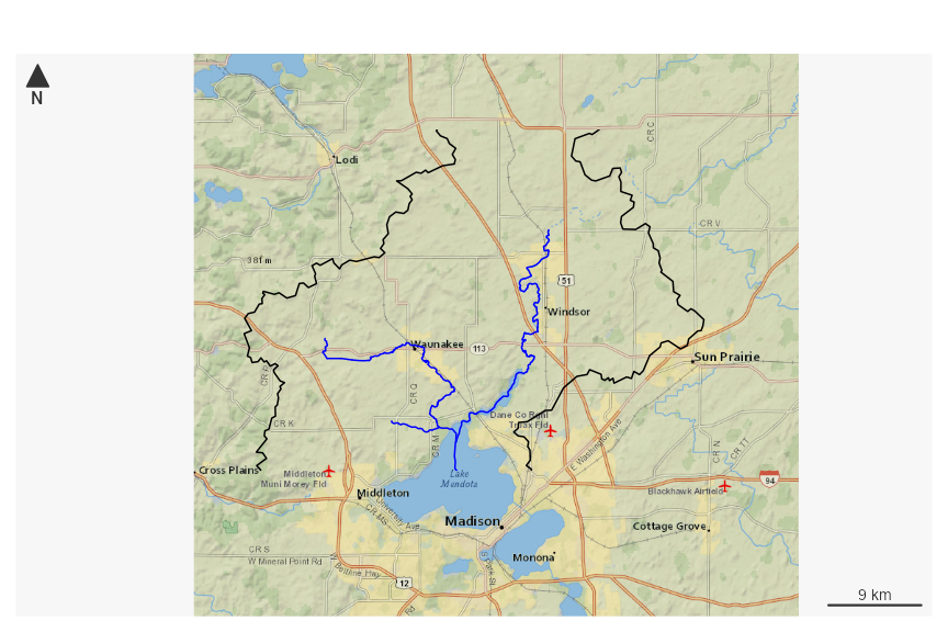
plot_nhdplus also allows modification of streamorder (if
you have data available locally) and styles. This plot request shows how
to get a subset of data for a plot and the range of options. See
documentation for more details.
source(system.file("extdata/sample_data.R", package = "nhdplusTools"))

plot_nhdplus(list(list("comid", "13293970"),
                  list("nwissite", "USGS-05428500"),
                  list("huc12pp", "070900020603"),
                  list("huc12pp", "070900020602")),
             streamorder = 2,
             nhdplus_data = sample_data,
             plot_config = list(basin = list(lwd = 2),
                                outlets = list(huc12pp = list(cex = 1.5),
                                               comid = list(col = "green"))))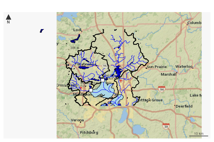
We can also plot NHDPlus data without an outlet at all.
bbox <- sf::st_bbox(c(xmin = -89.56684, ymin = 42.99816, xmax = -89.24681, ymax = 43.17192),
                    crs = "+proj=longlat +datum=WGS84 +no_defs")
plot_nhdplus(bbox = bbox)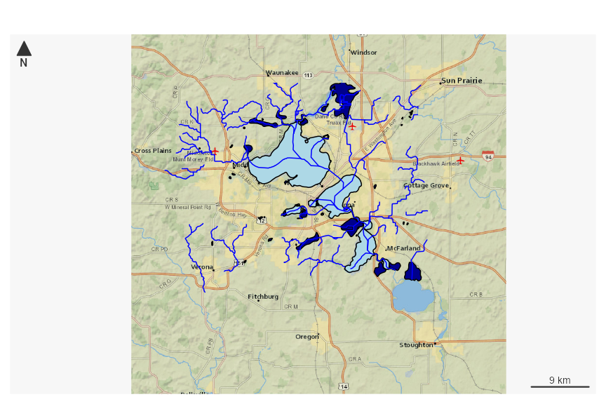
The plots above are all in the EPSG:3857 projection to be compatible with background tiles. Any data added to these plots must be projected to this coordinate system to be added to the plot.
Getting Data
What follows shows how to use nhdplusTools to create
plots without the plot_nhdplus function. While super
convenient, we all know the “easy button” is never quite right, the
description below should help get you started.
For this example, we’ll start from an outlet NWIS Site. Note that
other options are possible with discover_nhdplus_id and
dataRetrieval::get_nldi_sources.
library(sf)
library(nhdplusTools)
nwissite <- list(featureSource = "nwissite",
                     featureID = "USGS-05428500")

flowline <- navigate_nldi(nwissite,
                          mode = "upstreamTributaries",
                          data_source = "flowlines")

nhdplus <- subset_nhdplus(comids = as.integer(flowline$UT$nhdplus_comid),
                          output_file = file.path(work_dir, "nhdplus.gpkg"),
                          nhdplus_data = "download",
                          overwrite = TRUE, return_data = FALSE)

flowline <- read_sf(nhdplus, "NHDFlowline_Network")

upstream_nwis <- navigate_nldi(nwissite,
                               mode = "upstreamTributaries",
                               data_source = "nwissite")

basin <- get_nldi_basin(nwissite)
Now we have a file at the path held in the variable
nhdplus and three sf data.frames
with contents that look like:
st_layers(nhdplus)
#> Driver: GPKG
#> Available layers:
#>            layer_name geometry_type features fields crs_name
#> 1 NHDFlowline_Network   Line String       10    138    NAD83
names(flowline)
#>   [1] "objectid"     "comid"        "fdate"        "resolution"   "gnis_id"
#>   [6] "gnis_name"    "lengthkm"     "reachcode"    "flowdir"      "wbareacomi"
#>  [11] "ftype"        "fcode"        "shape_length" "streamleve"   "streamorde"
#>  [16] "streamcalc"   "fromnode"     "tonode"       "hydroseq"     "levelpathi"
#>  [21] "pathlength"   "terminalpa"   "arbolatesu"   "divergence"   "startflag"
#>  [26] "terminalfl"   "dnlevel"      "uplevelpat"   "uphydroseq"   "dnlevelpat"
#>  [31] "dnminorhyd"   "dndraincou"   "dnhydroseq"   "frommeas"     "tomeas"
#>  [36] "rtndiv"       "vpuin"        "vpuout"       "areasqkm"     "totdasqkm"
#>  [41] "divdasqkm"    "tidal"        "totma"        "wbareatype"   "pathtimema"
#>  [46] "hwnodesqkm"   "maxelevraw"   "minelevraw"   "maxelevsmo"   "minelevsmo"
#>  [51] "slope"        "elevfixed"    "hwtype"       "slopelenkm"   "qa_ma"
#>  [56] "va_ma"        "qc_ma"        "vc_ma"        "qe_ma"        "ve_ma"
#>  [61] "qa_01"        "va_01"        "qc_01"        "vc_01"        "qe_01"
#>  [66] "ve_01"        "qa_02"        "va_02"        "qc_02"        "vc_02"
#>  [71] "qe_02"        "ve_02"        "qa_03"        "va_03"        "qc_03"
#>  [76] "vc_03"        "qe_03"        "ve_03"        "qa_04"        "va_04"
#>  [81] "qc_04"        "vc_04"        "qe_04"        "ve_04"        "qa_05"
#>  [86] "va_05"        "qc_05"        "vc_05"        "qe_05"        "ve_05"
#>  [91] "qa_06"        "va_06"        "qc_06"        "vc_06"        "qe_06"
#>  [96] "ve_06"        "qa_07"        "va_07"        "qc_07"        "vc_07"
#> [101] "qe_07"        "ve_07"        "qa_08"        "va_08"        "qc_08"
#> [106] "vc_08"        "qe_08"        "ve_08"        "qa_09"        "va_09"
#> [111] "qc_09"        "vc_09"        "qe_09"        "ve_09"        "qa_10"
#> [116] "va_10"        "qc_10"        "vc_10"        "qe_10"        "ve_10"
#> [121] "qa_11"        "va_11"        "qc_11"        "vc_11"        "qe_11"
#> [126] "ve_11"        "qa_12"        "va_12"        "qc_12"        "vc_12"
#> [131] "qe_12"        "ve_12"        "lakefract"    "surfarea"     "rareahload"
#> [136] "rpuid"        "vpuid"        "enabled"      "geom"
names(upstream_nwis)
#> [1] "origin"      "UT_nwissite"
names(basin)
#> [1] "geometry"
class(st_geometry(flowline))
#> [1] "sfc_LINESTRING" "sfc"
class(st_geometry(upstream_nwis$UT_nwissite))
#> [1] "sfc_POINT" "sfc"
class(st_geometry(basin))
#> [1] "sfc_POLYGON" "sfc"
Our file has four layers: network flowlines, simplified catchments, nhd area features, and nhd waterbody features.
The flowlines have a large set of attributes from the NHDPlus
dataset. And the nwis sites have a few attributes that came from the
NLDI. Attributes for NWIS sites can be found using the dataRetrieval
package.
See the NHDPlus user guide linked here for more on what these layers are and what the flowline attributes entail.
Base R Plotting
In order to maximize flexibility and make sure we understand what’s
going on with coordinate reference systems, the demonstration below
shows how to use base R plotting with the package mapsf and
maptiles.
In this example, we have to plot just the geometry, extracted with
st_geometry and we need to project the geometry into the
plotting coordinate reference system, EPSG:3857 also known
as “web mercator”. The reason we have to make this transformation is
that practically all basemap tiles are in this projection and
reprojection of pre-rendered tiles doesn’t look good. We do this with a
simple prep_layer function.
The mapsf, maptiles, and base
plot commands put data onto the R plotting device so the
first to be plotted is on the bottom. A couple hints here.
lwd is line width. pch is point style.
cex is an expansion factor. Colors shown below are basic R
colors. the rgb function is handy for creating colors with
transparency if that’s of interest.
prep_layer <- function(x) st_geometry(st_transform(x, 3857))

bb <- sf::st_as_sfc(sf::st_bbox(prep_layer(basin)))

tiles <- maptiles::get_tiles(bb,
                             zoom = 11, crop = FALSE,
                             verbose = FALSE,
                             provider = "Esri.NatGeoWorldMap")

mapsf::mf_map(bb, type = "base", col = NA, border = NA)

maptiles::plot_tiles(tiles, add = TRUE)

mapsf::mf_map(bb, type = "base", add = TRUE, col = NA, border = NA)
mapsf::mf_arrow(align = bb)
mapsf::mf_scale()

plot(prep_layer(basin),
     lwd = 2, add = TRUE)

plot(prep_layer(flowline),
     lwd = 1.5, col = "deepskyblue", add = TRUE)

plot(prep_layer(dplyr::filter(flowline, streamorde > 2)),
     lwd = 3, col = "darkblue", add = TRUE)

us_nwis_layer <- prep_layer(upstream_nwis$UT_nwissite)

plot(us_nwis_layer,
     pch = 17, cex = 1.5, col = "yellow", add = TRUE)

label_pos <- st_coordinates(us_nwis_layer)

text(label_pos[,1],label_pos[,2],
     upstream_nwis$identifier,
     adj = c(-0.2, 0.5), cex = 0.7)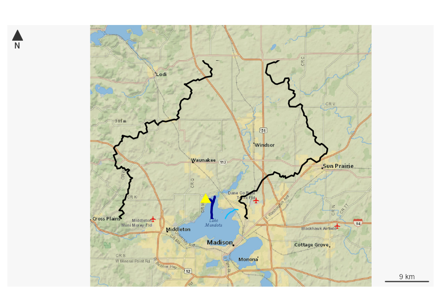
Plotting with ggplot2
Below is a very similar example using ggmap and ggplot2
geom_sf. Note that ggmap takes case of projections for
us, which should either make you happy because it just works or
very nervous because it just works.
library(ggmap)
library(ggplot2)

ggmap_bbox <- setNames(sf::st_bbox(basin), c("left", "bottom", "right", "top"))
ggmap_bbox
#>      left    bottom     right       top
#> -89.60465  43.03507 -89.20378  43.36607

upstream_nwis <- dplyr::bind_cols(upstream_nwis$UT_nwissite,
                           dplyr::rename(dplyr::as_tibble(sf::st_coordinates(upstream_nwis$UT_nwissite)),
                                         lat = Y, lon = X))

# ggmap now requires api keys
# basemap_toner <- get_map(source = "stamen", maptype = "toner",
#                          location = ggmap_bbox, zoom = 11, messaging = FALSE)
# basemap_terrain <- get_map(source = "stamen", maptype = "terrain-lines",
#                            location = ggmap_bbox, zoom = 11, messaging = FALSE)
# toner_map <- ggmap(basemap_toner)
# terrain_map <- ggmap(basemap_terrain)
#
# toner_map

ggplot() + geom_sf(data = basin,
                        inherit.aes = FALSE,
                        color = "black", fill = NA) +
  geom_sf(data = flowline,
          inherit.aes = FALSE,
          color = "deepskyblue") +
  geom_sf(data = dplyr::filter(flowline, streamorde > 2),
          inherit.aes = FALSE,
          color = "darkblue") +
  geom_sf(data = upstream_nwis, inherit.aes = FALSE, color = "red") +
  geom_text(data = upstream_nwis, aes(label = identifier, x = lon, y = lat),
            hjust = 0, size=2.5, nudge_x = 0.02, col = "black")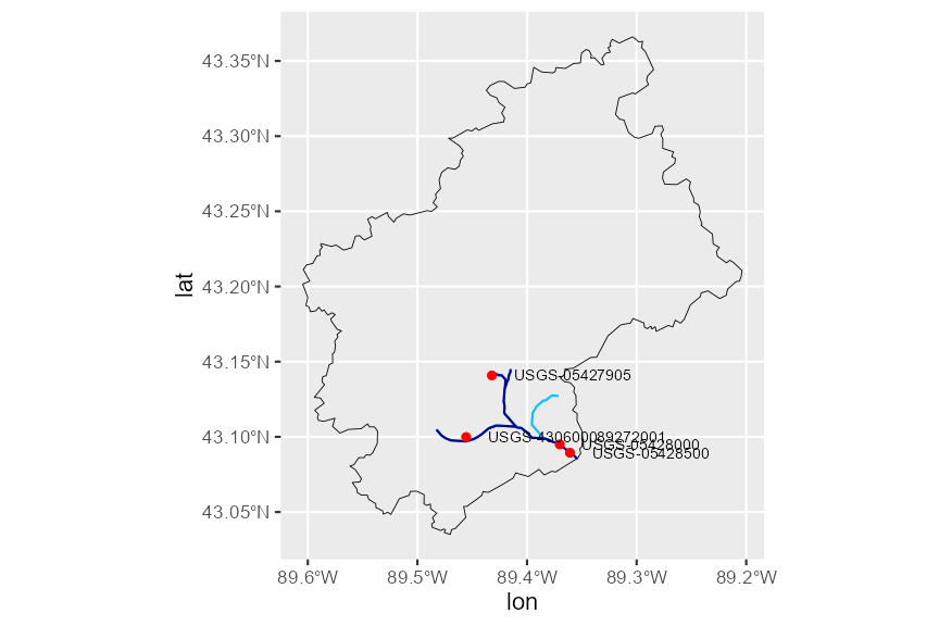
Hopefully these examples give a good head start to plotting NHDPlus data. Please submit questions via github issues for more!! Pull requests on this vignette are more than welcome if you have additions or suggestions.