NHDPlusTools Data Access Overview
dblodgett@usgs.gov
Source:vignettes/get_data_overview.Rmd
get_data_overview.RmdSince it’s original release in 2019, data access in nhdplusTools has evolved and grown considerably. This vignette, prepared for a workshop in Summer 2024 shows the diversity of data available with nhdplusTools in one holistic overview.
The function naming in nhdplusTools related to data
access uses three common terms:
1. “download” will generally download complete data sets for use
locally. 2. “get” will pull a data subset from a web service. 3.
“subset” will pull a subset from a local file and, when available, a web
service.
Dataset function index.
The following summarizes specific data access functions available for
the datasets that nhdplusTools has supporting functionality
for.
- NHDPlusV2
-
download_nhdplusv2()- downloads a National seamless geodatabase -
get_nhdplus()- access NHDPlusV2 from a web service -
subset_nhdplus()- subsets the National geodatabase OR the web service -
subset_rpu()- subsets loaded NHDPlusV2 by raster processing unit -
subset_vpu()- subsets loaded NHDPlusV2 by vector processing unit -
get_boundaries()- retrieves NHDPlusV2 processing unit boundaries
-
- NHDPlusHR
-
download_nhdplushr()- downloads staged geodatabases -
get_nhdplushr()- assembles nhdplushr datasets from many staged databases -
get_hr_data()- helps pull data out of staged databases (used byget_nhdplushr())
-
- NHD
-
download_nhd()- downloads staged geodatabases
-
- 3DHP
-
get_3dhp- access 3DHP from a web service
-
- geoconnex
-
get_geoconnex_reference()- access geoconnex reference features from a web service
-
- WBD
-
download_wbd()- download a National WBD geodatabase -
get_huc()- get a particular Hydrologic Unit Code from a service
-
- RF1
-
download_rf1()- download a National RF1 geodatabase
-
Network Linked Data Index integration
The Network Linked Data Index plays a key role in discovery
nhdplusTools. It provides access to an easy network
navigation and basin boundary delineation tool. Behind the scenes, the
NLDI is based on the network of the NHDPlusV2 – so has some special
functionality related directly to that dataset. Functions that utilize
the NLDI include:
subset_nhdplus()plot_nhdplus()map_nhdplus()discover_nhdplus_id()get_nldi_basin()get_nldi_feature()get_nldi_index()navigate_network()navigate_nldi()get_split_catchment()get_raindrop_trace()
In the demo below, we’ll choose a stream gage and show how to access data related to it from all the datasets that nhdplusTools works with as well as use some of the NLDI functionality in question.
For the sake of demonstration, we’ll look at the Wolf River at Langlade, WI – site ID “04074950”.
nhdplusTools allows us to start from a stream gage to build a subset of NHDPlusV2 data. Below, we’ll do just that and plot the results on a default map.
demo_dir <- nhdplusTools_data_dir()

site_id <- "USGS-04074950"


# use dataRetrieval::get_nldi_sources() to find other nldi sources

site <- list(featureSource = "nwissite",
             featureID = "USGS-04074950")

site_feature <- get_nldi_feature(site)

upstream_network <- navigate_nldi(site,
                                  mode = "UT", distance_km = 9999)

demo_data <- file.path(demo_dir, "data_demo.gpkg")

dataset <- subset_nhdplus(as.integer(upstream_network$UT_flowlines$nhdplus_comid),
                          nhdplus_data = "download", # download from a service
                          output_file = demo_data, # write the data to disk
                          return_data = TRUE, # return the data rather
                          flowline_only = FALSE, overwrite = TRUE)

names(dataset)
#> [1] "NHDFlowline_Network"    "CatchmentSP"            "NHDArea"
#> [4] "NHDWaterbody"           "NHDFlowline_NonNetwork"

sapply(dataset, nrow)
#>    NHDFlowline_Network            CatchmentSP                NHDArea
#>                    389                    370                     20
#>           NHDWaterbody NHDFlowline_NonNetwork
#>                    473                      8

old_par <- par(mar = c(0, 0, 0, 0))

plot_nhdplus(outlets = list(featureSource = "nwissite",
                            featureID = "USGS-04074950"),
             nhdplus_data = demo_data, flowline_only = TRUE)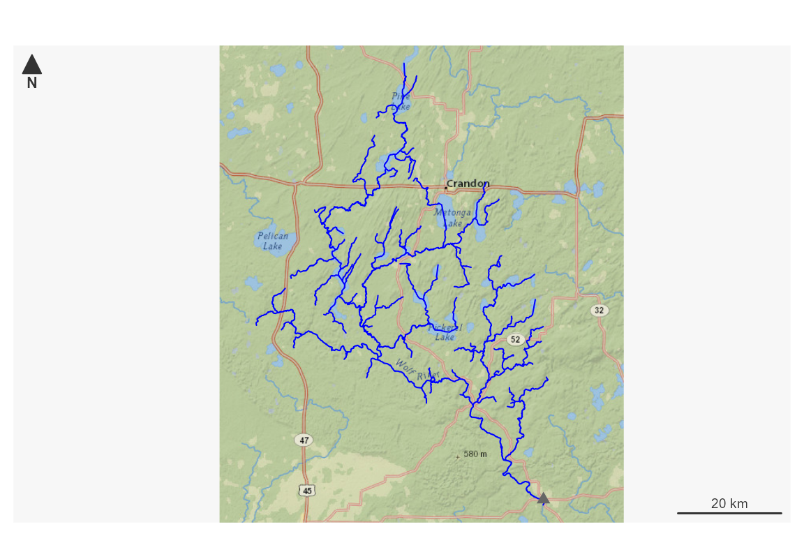
The above is the original way NHDPlusTools supported access NHDPlusV2
data. A dedicated web service subset utility is available in
get_nhdplus – which is what subset_nhdplus()
calls behind the scenes.
Here we grab the basin for our site and request NHDPlus with its geometry as the Area of Interest.
basin <- get_nldi_basin(site)

subset <- get_nhdplus(AOI = basin, realization = "flowline")

par(mar = c(0, 0, 0, 0))

plot(sf::st_geometry(basin))
plot(sf::st_geometry(subset), col = "blue", add = TRUE)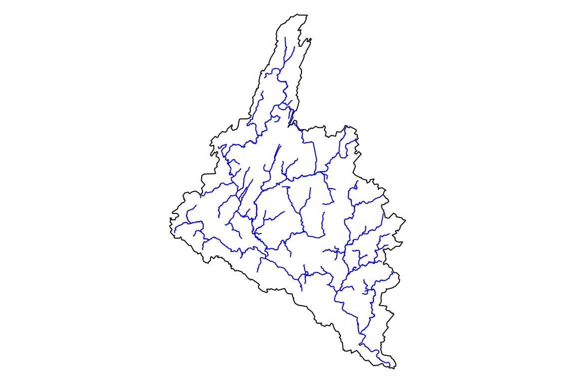
For NHDPlusHR data, which is much denser than NHDPlusV2,
nhdplusTools supports downloading four-digit Hydrologic
Unit Code staged geodatabases. The function get_huc() is
useful to discover the code needed here.
wolf_huc <- get_huc(basin, type = 'huc04')
#> defaulting to 2025 version of WBD

nrow(wolf_huc)
#> [1] 2

# it straddles hucs? Not really.

par(mar = c(0, 0, 0, 0))
plot(sf::st_geometry(basin), col = "grey")
plot(sf::st_geometry(wolf_huc), add = TRUE)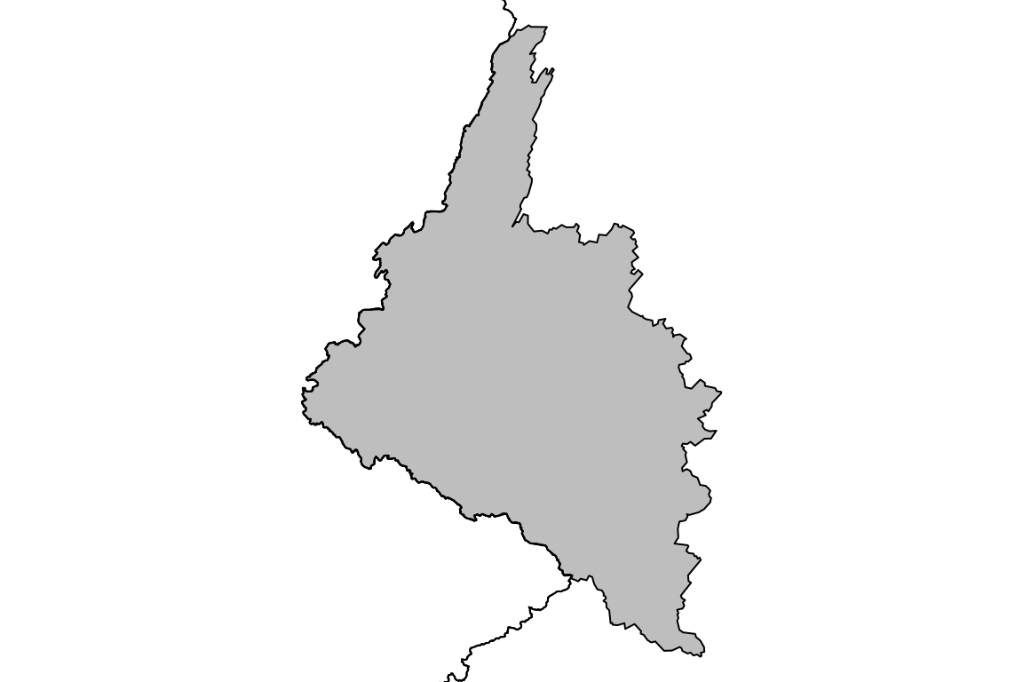
wolf_huc <- get_huc(site_feature, type = "huc04")
#> defaulting to 2025 version of WBD

nrow(wolf_huc)
#> [1] 1

# better!!
par(mar = c(0, 0, 0, 0))
plot(sf::st_geometry(wolf_huc))
plot(sf::st_geometry(basin), col = "grey", add = TRUE)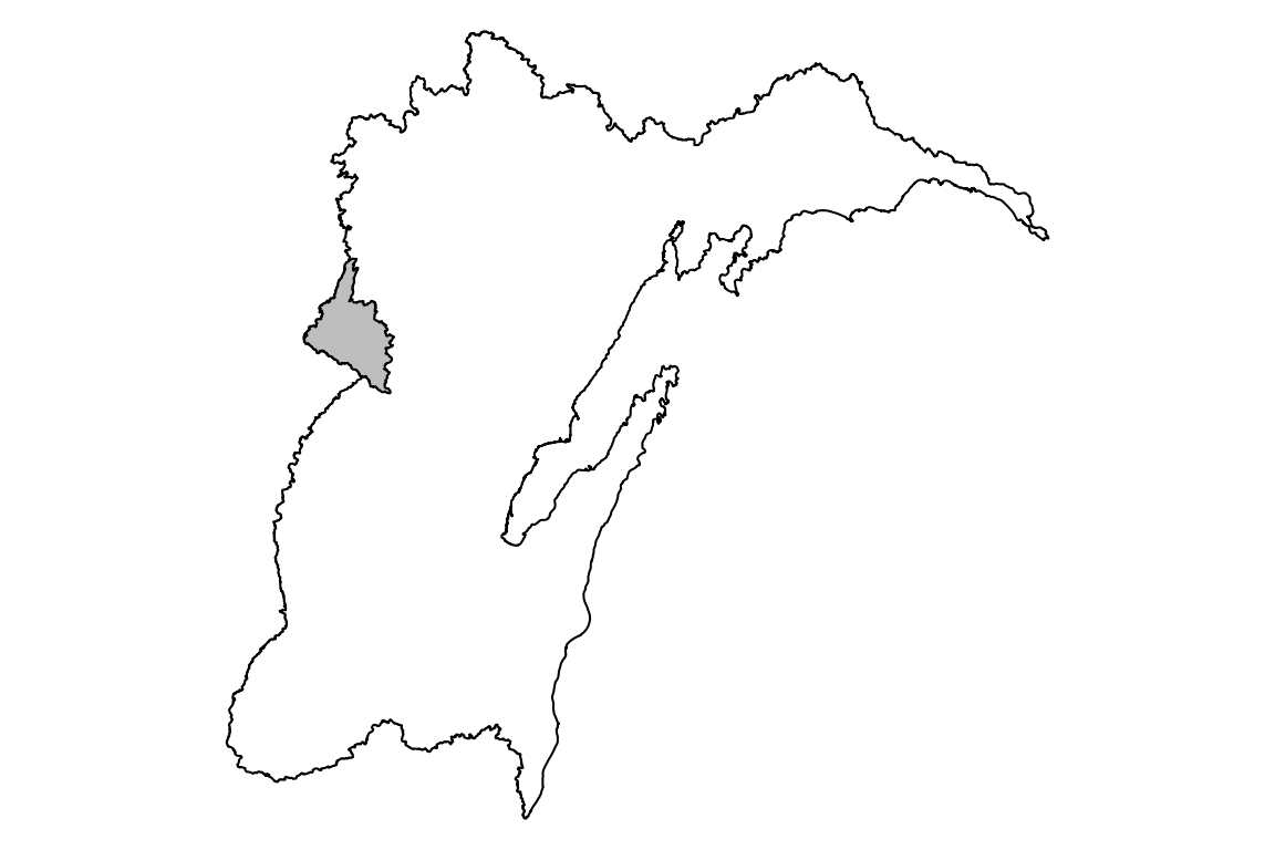
outdir <- file.path(nhdplusTools_data_dir(), "hr_access_demo")

dir.create(outdir)
#> Warning in dir.create(outdir):
#> 'C:\Users\dblodgett\AppData\Roaming\R\data\R\nhdplusTools\hr_access_demo'
#> already exists

download_dir <- download_nhdplushr(outdir, wolf_huc$huc4)

list.files(download_dir)
#> [1] "NHDPLUS_H_0403_HU4_GDB.gdb" "NHDPLUS_H_0403_HU4_GDB.jpg"
#> [3] "NHDPLUS_H_0403_HU4_GDB.xml"
If we had asked for more HUC4 codes, additional gdb files would be in the directory we specified.
With this, we can use one of the two functions for access NHDPlusHR
data to load data from the directory. Here, we use the more complete
get_nhdplus() and set check_terminals=TRUE
which uses make_standalone() to ensure that the nhdplus
attributes are complete and self-consistent within the subset of data
returned.
nhdplushr <- get_nhdplushr(
  download_dir,
  layers = c("NHDFlowline", "NHDPlusCatchment", "NHDWaterbody",
             "NHDArea", "NHDLine", "NHDPlusSink", "NHDPlusWall",
             "NHDPoint", "NHDPlusBurnWaterbody", "NHDPlusBurnLineEvent",
             "HYDRO_NET_Junctions", "WBDHU2", "WBDHU4","WBDHU6",
             "WBDHU8", "WBDHU10", "WBDHU12", "WBDLine"),
  check_terminals = TRUE)
#> Warning in CPL_read_ogr(dsn, layer, query, as.character(options), quiet, : GDAL
#> Message 1: organizePolygons() received a polygon with more than 100 parts. The
#> processing may be really slow.  You can skip the processing by setting
#> METHOD=SKIP, or only make it analyze counter-clock wise parts by setting
#> METHOD=ONLY_CCW if you can assume that the outline of holes is counter-clock
#> wise defined

sapply(nhdplushr, nrow)
#>          NHDFlowline     NHDPlusCatchment         NHDWaterbody
#>                53834                51815                34138
#>              NHDArea              NHDLine          NHDPlusSink
#>                 1283                  207                  582
#>          NHDPlusWall             NHDPoint NHDPlusBurnWaterbody
#>                 2031                   73                25146
#> NHDPlusBurnLineEvent  HYDRO_NET_Junctions               WBDHU2
#>                51938                53555                    1
#>               WBDHU4               WBDHU6               WBDHU8
#>                    1                    2                   18
#>              WBDHU10              WBDHU12              WBDLine
#>                  107                  629                 2031
At a lower level, we can use get_hr_data() to access
particular layers. Here, rename=TRUE causes the nhdplushr
names to be normalized to nhdplusTools conventions using
align_nhdplus_names().
NOTE: “NHDPlusID” from nhdplushr is replaced with the name “COMID”. This attribute is merely a unique integer identifier and should not be assumed to relate to anything outside the context of a given dataset.
nhdplushr <- get_hr_data(list.files(download_dir, pattern = ".gdb", full.names = TRUE),
                         layer = "NHDFlowline", rename = TRUE)

names(nhdplushr)
#>  [1] "Permanent_Identifier"        "FDate"
#>  [3] "Resolution"                  "GNIS_ID"
#>  [5] "GNIS_Name"                   "LENGTHKM"
#>  [7] "REACHCODE"                   "FlowDir"
#>  [9] "WBArea_Permanent_Identifier" "FTYPE"
#> [11] "FCODE"                       "MainPath"
#> [13] "InNetwork"                   "VisibilityFilter"
#> [15] "Shape_Length"                "COMID"
#> [17] "VPUID"                       "Enabled"
#> [19] "Shape"                       "StreamLeve"
#> [21] "StreamOrde"                  "StreamCalc"
#> [23] "FromNode"                    "ToNode"
#> [25] "Hydroseq"                    "LevelPathI"
#> [27] "Pathlength"                  "TerminalPa"
#> [29] "ArbolateSu"                  "Divergence"
#> [31] "StartFlag"                   "TerminalFl"
#> [33] "UpLevelPat"                  "UpHydroseq"
#> [35] "DnLevel"                     "DnLevelPat"
#> [37] "DnHydroseq"                  "DnMinorHyd"
#> [39] "DnDrainCou"                  "FromMeas"
#> [41] "ToMeas"                      "RtnDiv"
#> [43] "Thinner"                     "VPUIn"
#> [45] "VPUOut"                      "AreaSqKM"
#> [47] "TotDASqKM"                   "DivDASqKm"
#> [49] "MaxElevRaw"                  "MinElevRaw"
#> [51] "MaxElevSmo"                  "MinElevSmo"
#> [53] "Slope"                       "SlopeLenKm"
#> [55] "ElevFixed"                   "HWType"
#> [57] "HWNodeSqKm"                  "StatusFlag"

# Great Lakes coast are flowlines -- remove for visuals
gl_coast <- c(get_DM(nhdplushr, 60002700000331),
              get_DM(nhdplushr, 60002700049157))
#> defaulting to comid rather than permanent_identifier
#> defaulting to comid rather than permanent_identifier

plot_data <- dplyr::filter(nhdplushr, FCODE != 56600 & StreamOrde > 2 & !COMID %in% gl_coast)

par(mar = c(0, 0, 0, 0))
plot(sf::st_geometry(wolf_huc))
plot(sf::st_geometry(basin), col = "grey", add = TRUE)
plot(sf::st_geometry(plot_data), lwd = plot_data$StreamOrde / 3, col = "blue", add = TRUE)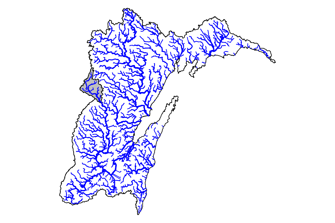
par(mar = c(0, 0, 0, 0))
plot(sf::st_geometry(basin), col = "grey")
plot(sf::st_geometry(plot_data), lwd = plot_data$StreamOrde / 2, col = "blue", add = TRUE)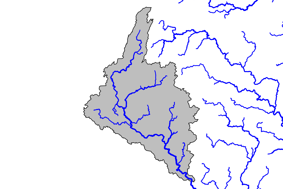 BONUS DEMO: Say we want to know where our stream gage is on the river in
question…
get_flowline_index() and
disambiguate_flowline_indexes() are your friends.
potential_matches <- get_flowline_index(nhdplushr,
                                        points = site_feature,
                                        search_radius = units::as_units(500, "m"),
                                        max_matches = 5)
#> defaulting to comid rather than permanent_identifier
#> Warning in match_crs(x, points, paste("crs of lines and points don't match.", :
#> crs of lines and points don't match. attempting st_transform of lines
#> Warning in force_linestring(x): converting to LINESTRING, this may be slow,
#> check results

potential_matches
#>   id          COMID      REACHCODE REACH_meas       offset
#> 1  1 60002700035364 04030202000126    34.9737 0.0002166323
#> 2  1 60002700000908 04030104001542    49.1370 0.0177673341
#> 3  1 60002700036849 04030104001542    81.5378 0.0224609122
#> 4  1 60002700035750 04030104000533    31.4940 0.0244823037
#> 5  1 60002700034888 04030104000136   100.0000 0.0247855142

site_meta <- dataRetrieval::readNWISsite(gsub("USGS-", "", site_feature$identifier))
#> Warning in dataRetrieval::readNWISsite(gsub("USGS-", "",
#> site_feature$identifier)): NWIS servers are slated for decommission. Please
#> begin to migrate to read_waterdata_monitoring_location
#> GET: https://waterservices.usgs.gov/nwis/site/?siteOutput=Expanded&format=rdb&site=04074950

sqmi_to_sqkm <- 2.59

da_df <- data.frame(id = 1, drainagearea = site_meta$drain_area_va * sqmi_to_sqkm)

# uses nearest drainage area match
disambiguate_flowline_indexes(potential_matches,
                              flowpath = dplyr::select(nhdplushr, COMID, TotDASqKM),
                              hydro_location = da_df)
#> # A tibble: 1 × 5
#>      id   COMID REACHCODE      REACH_meas   offset
#>   <dbl>   <dbl> <chr>               <dbl>    <dbl>
#> 1     1 6.00e13 04030202000126       35.0 0.000217
If what you really need is the base NHD, which is now a static
dataset, the pattern is just the same as with nhdplushr using
download_nhd().
outdir <- file.path(nhdplusTools_data_dir(), "nhd_access_demo")

dir.create(outdir)
#> Warning in dir.create(outdir):
#> 'C:\Users\dblodgett\AppData\Roaming\R\data\R\nhdplusTools\nhd_access_demo'
#> already exists

download_dir <- download_nhd(outdir, wolf_huc$huc4)

list.files(download_dir)
#> [1] "NHD_H_0403_HU4_GDB.gdb" "NHD_H_0403_HU4_GDB.jpg" "NHD_H_0403_HU4_GDB.xml"

nhd_gdb <- list.files(download_dir, pattern = ".gdb", full.names = TRUE)

sf::st_layers(nhd_gdb)
#> Driver: OpenFileGDB
#> Available layers:
#>                 layer_name                 geometry_type features fields
#> 1        ExternalCrosswalk                            NA        1      6
#> 2                 NHDFCode                            NA      126     13
#> 3     NHDFeatureToMetadata                            NA   277698      2
#> 4                  NHDFlow                            NA    67048      4
#> 5           NHDFlowlineVAA                            NA    53733     22
#> 6              NHDMetadata                            NA      312     21
#> 7  NHDProcessingParameters                            NA        5      2
#> 8  NHDReachCodeMaintenance                            NA    62818      6
#> 9   NHDReachCrossReference                            NA    78278     11
#> 10       NHDSourceCitation                            NA      350     13
#> 11               NHDStatus                            NA        0      3
#> 12 NHDVerticalRelationship                            NA        0      3
#> 13                CLIPPOLY                 Multi Polygon        0      2
#> 14            NHDWaterbody              3D Multi Polygon    34143     13
#> 15         NHDPointEventFC                         Point     2705     14
#> 16                NHDPoint                      3D Point       74      8
#> 17          NHDLineEventFC             Multi Line String        0     16
#> 18                 NHDLine          3D Multi Line String      207     10
#> 19             NHDFlowline 3D Measured Multi Line String    53850     16
#> 20          NHDAreaEventFC                 Multi Polygon        0     14
#> 21                 NHDArea              3D Multi Polygon     1283     12
#> 22                 WBDLine             Multi Line String     2970      7
#> 23                  WBDHU8                 Multi Polygon       18     14
#> 24                  WBDHU6                 Multi Polygon        2     14
#> 25                  WBDHU4                 Multi Polygon        1     14
#> 26                  WBDHU2                 Multi Polygon        1     14
#> 27                 WBDHU16                 Multi Polygon        0     19
#> 28                 WBDHU14                 Multi Polygon        0     19
#> 29                 WBDHU12                 Multi Polygon      629     19
#> 30                 WBDHU10                 Multi Polygon      107     16
#> 31     HYDRO_NET_Junctions                         Point    53573      1
#> 32      HYDRO_NET_BUILDERR                            NA       21      3
#> 33                N_1_Desc                            NA   107423      5
#> 34               N_1_EDesc                            NA       40      2
#> 35             N_1_EStatus                            NA        1      2
#> 36               N_1_ETopo                            NA       14      2
#> 37              N_1_FloDir                            NA        1      2
#> 38               N_1_JDesc                            NA       40      2
#> 39             N_1_JStatus                            NA        1      2
#> 40               N_1_JTopo                            NA      105      2
#> 41              N_1_JTopo2                            NA        1      2
#> 42               N_1_Props                            NA        9      2
#>                 crs_name
#> 1                   <NA>
#> 2                   <NA>
#> 3                   <NA>
#> 4                   <NA>
#> 5                   <NA>
#> 6                   <NA>
#> 7                   <NA>
#> 8                   <NA>
#> 9                   <NA>
#> 10                  <NA>
#> 11                  <NA>
#> 12                  <NA>
#> 13                 NAD83
#> 14 NAD83 + NAVD88 height
#> 15 NAD83 + NAVD88 height
#> 16 NAD83 + NAVD88 height
#> 17 NAD83 + NAVD88 height
#> 18 NAD83 + NAVD88 height
#> 19 NAD83 + NAVD88 height
#> 20 NAD83 + NAVD88 height
#> 21 NAD83 + NAVD88 height
#> 22                 NAD83
#> 23                 NAD83
#> 24                 NAD83
#> 25                 NAD83
#> 26                 NAD83
#> 27                 NAD83
#> 28                 NAD83
#> 29                 NAD83
#> 30                 NAD83
#> 31 NAD83 + NAVD88 height
#> 32                  <NA>
#> 33                  <NA>
#> 34                  <NA>
#> 35                  <NA>
#> 36                  <NA>
#> 37                  <NA>
#> 38                  <NA>
#> 39                  <NA>
#> 40                  <NA>
#> 41                  <NA>
#> 42                  <NA>

nhd_fline <- sf::read_sf(nhd_gdb, "NHDFlowline")
We’ll wait to plot this up until after we’ve done some work with
3DHP. As of writing, the 3DHP is more or less the same as the NHD but in
a new database schema. The get_3dhp() uses a web service to
pull data for subsets much the same as the other get_*
functions. See vignette("get_3dhp_data.Rmd") for more on
how to work with 3DHP data.
sub_3dhp <- get_3dhp(basin, type = "flowline")
#> Getting features 0 to 2000 of 2199
#> Getting features 2000 to 2199 of 2199

plot(sub_3dhp)
#> Warning: plotting the first 10 out of 34 attributes; use max.plot = 34 to plot
#> all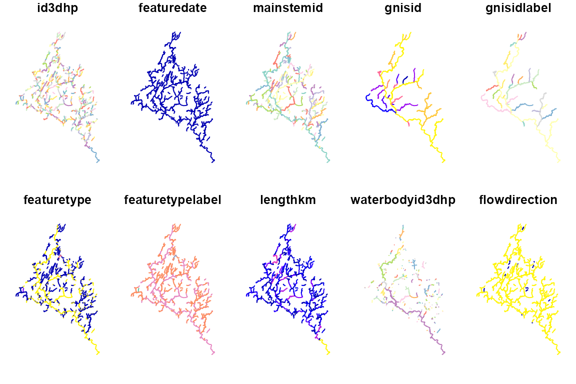
sub_3dhp <- st_compatibalize(sub_3dhp, nhd_fline)

par(mar = c(0, 0, 0, 0))
plot(sf::st_geometry(basin), col = "grey")
plot(sf::st_geometry(sf::st_zm(sub_3dhp)), col = "skyblue", lwd = 2.5, add = TRUE)
plot(sf::st_geometry(sf::st_zm(nhd_fline)), col = "blue", lwd = 0.1, add = TRUE)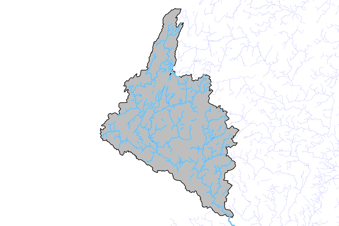
A brand new, May 2024, feature in nhdplusTools is access to the
geoconnex.us reference feature server. The reference feature server
provides easy access to representations of datasets that people use to
cross reference other data. discover_geoconnex_reference()
provides access to a full table of what’s available.
unique(discover_geoconnex_reference()[c("id", "title")])
#> # A tibble: 18 × 2
#>    id            title
#>    <chr>         <chr>
#>  1 hu02          HU02
#>  2 hu04          HU04
#>  3 hu06          HU06
#>  4 hu08          HU08
#>  5 hu10          HU10
#>  6 nat_aq        USGS National Aquifers
#>  7 principal_aq  USGS Principal Aquifers
#>  8 sec_hydrg_reg USGS Secondary Hydrogeologic Regions
#>  9 gages         Reference Gages
#> 10 mainstems     Reference Mainstems
#> 11 dams          Reference Dams
#> 12 pws           Public Water Systems
#> 13 states        States
#> 14 counties      Counties
#> 15 aiannh        American Indian/Alaska Native Areas/Hawaiian Home Lands
#> 16 cbsa          Core-based statistical areas
#> 17 ua10          Urban Areas
#> 18 places        Places
Each of these sets of “reference features” includes a “uri” which is a persistent way to identify these features and will always lead you back to a representation of the feature when you look it up.
For example, let’s get a subset of data for our Wolf River basin.
wolf_gages <- get_geoconnex_reference(basin, type = "gages")
geoconnex_gage <- dplyr::filter(wolf_gages,
provider_id == site_feature$identifier)
wolf_mainstems <- get_geoconnex_reference(basin, type = "mainstems")
wolf_mainstem <- dplyr::filter(wolf_mainstems, uri == geoconnex_gage$mainstem_uri)
par(mar = c(0, 0, 0, 0))
plot(sf::st_geometry(basin), col = "grey")
plot(sf::st_geometry(wolf_mainstems), lwd = 0.5, col = "blue", add = TRUE)
plot(sf::st_geometry(wolf_mainstem), lwd = 3, col = "blue", add = TRUE)
plot(sf::st_geometry(wolf_gages), pch = 2, cex = 0.75, add = TRUE)
plot(sf::st_geometry(geoconnex_gage), pch = 17, cex = 1.5, add = TRUE)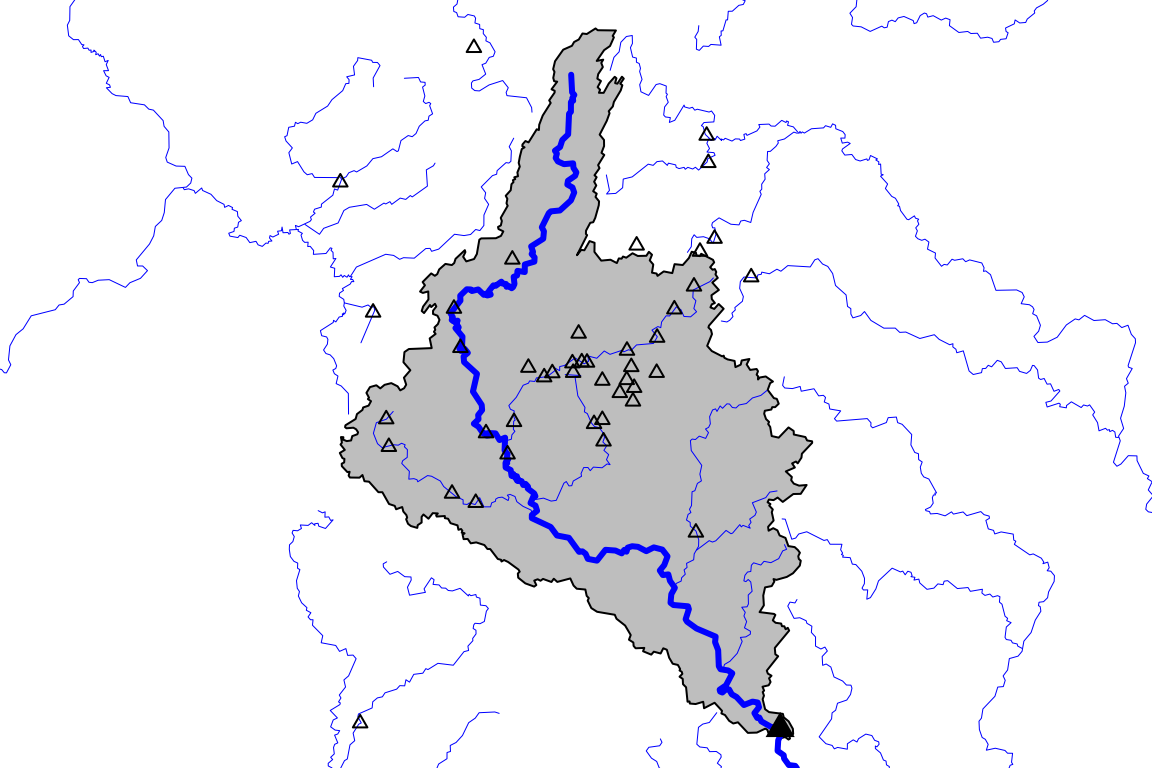 The Watershed Boundary Dataset contains hydrologic units that are used
as cataloging units for the country. It was developed and improved over
the last twenty years and is nearing a complete static state. There are
three prominent versions of it available – a snapshot available as part
of the NHDPlusV2, a snapshot available as part of and retrieved with
get_huc(), and the latest (soon to be final) snapshot
available using download_wbd().
wbd_dir <- file.path(nhdplusTools_data_dir(), "wbd_access_demo")

wbd_out <- download_wbd(wbd_dir)
#> Compressed WBD file already exists ...
#> Extracting data ...
#> Error in zip::unzip(file, exdir = outdir, overwrite = FALSE) :
#>   zip error: Cannot open zip file `C:\Users\dblodgett\AppData\Roaming\R\data\R\nhdplusTools\wbd_access_demo\WBD_National_GDB.zip` for reading in file zip.c:144
#> WBD data extracted to: C:\Users\dblodgett\AppData\Roaming/R/data/R/nhdplusTools/wbd_access_demo/WBD_National_GDB.gdb

# zip::unzip doesn't always work
if(length(wbd_out == 0)) {
  f <- list.files(wbd_dir, pattern = ".zip", full.names = TRUE)

  utils::unzip(f, exdir = wbd_dir)
}

wbd_gdb <- list.files(wbd_dir, pattern = ".gdb", full.names = TRUE)

sf::st_layers(wbd_gdb)
#> Driver: OpenFileGDB
#> Available layers:
#>                     layer_name     geometry_type features fields
#> 1                      WBDHU12     Multi Polygon   103025     20
#> 2             NWISDrainageLine Multi Line String   127876     12
#> 3                       WBDHU8     Multi Polygon     2413     15
#> 4  NonContributingDrainageLine Multi Line String        0     10
#> 5                       WBDHU4     Multi Polygon      245     15
#> 6                      WBDHU16     Multi Polygon     7202     20
#> 7  NonContributingDrainageArea     Multi Polygon        0     12
#> 8             NWISDrainageArea     Multi Polygon     2733     19
#> 9                       WBDHU6     Multi Polygon      405     15
#> 10                      WBDHU2     Multi Polygon       22     15
#> 11                     WBDHU14     Multi Polygon     8138     20
#> 12                     WBDLine Multi Line String   394965      8
#> 13                     WBDHU10     Multi Polygon    18867     17
#> 14           FeatureToMetadata                NA   564839      3
#> 15           ExternalCrosswalk                NA        0      7
#> 16                       HUMod                NA       23      5
#> 17           MetaProcessDetail                NA     1850     16
#> 18            MetaSourceDetail                NA     1854     27
#> 19        ProcessingParameters                NA        2      2
#> 20                UpdateStatus                NA        0      2
#>                 crs_name
#> 1  NAD83 + NAVD88 height
#> 2  NAD83 + NAVD88 height
#> 3  NAD83 + NAVD88 height
#> 4  NAD83 + NAVD88 height
#> 5  NAD83 + NAVD88 height
#> 6  NAD83 + NAVD88 height
#> 7  NAD83 + NAVD88 height
#> 8  NAD83 + NAVD88 height
#> 9  NAD83 + NAVD88 height
#> 10 NAD83 + NAVD88 height
#> 11 NAD83 + NAVD88 height
#> 12 NAD83 + NAVD88 height
#> 13 NAD83 + NAVD88 height
#> 14                  <NA>
#> 15                  <NA>
#> 16                  <NA>
#> 17                  <NA>
#> 18                  <NA>
#> 19                  <NA>
#> 20                  <NA>