TL;DR
Pick an outlet location and download some data.
# Uncomment to install!
# install.packages("nhdplusTools")

library(nhdplusTools)
library(sf)

start_point <- st_sfc(st_point(c(-89.362239, 43.090266)), crs = 4269)
start_comid <- discover_nhdplus_id(start_point)

flowline <- navigate_nldi(list(featureSource = "comid",
                               featureID = start_comid),
                          mode = "upstreamTributaries",
                          distance_km = 1000)

subset_file <- tempfile(fileext = ".gpkg")
subset <- subset_nhdplus(comids = as.integer(flowline$UT$nhdplus_comid),
                         output_file = subset_file,
                         nhdplus_data = "download",
                         flowline_only = FALSE,
                         return_data = TRUE, overwrite = TRUE)
#> All intersections performed in latitude/longitude.
#> Reading NHDFlowline_Network
#> Spherical geometry (s2) switched off
#> Spherical geometry (s2) switched on
#> Writing NHDFlowline_Network
#> Reading CatchmentSP
#> Spherical geometry (s2) switched off
#> Spherical geometry (s2) switched on
#> Writing CatchmentSP
#> Spherical geometry (s2) switched off
#> although coordinates are longitude/latitude, st_intersects assumes that they
#> are planar
#> Spherical geometry (s2) switched on
#> Spherical geometry (s2) switched off
#> although coordinates are longitude/latitude, st_intersects assumes that they
#> are planar
#> Spherical geometry (s2) switched on
#> Spherical geometry (s2) switched off
#> although coordinates are longitude/latitude, st_intersects assumes that they
#> are planar
#> Spherical geometry (s2) switched on

flowline <- subset$NHDFlowline_Network
catchment <- subset$CatchmentSP
waterbody <- subset$NHDWaterbody

## Or using a file:

flowline <- sf::read_sf(subset_file, "NHDFlowline_Network")
catchment <- sf::read_sf(subset_file, "CatchmentSP")
waterbody <- sf::read_sf(subset_file, "NHDWaterbody")

plot(sf::st_geometry(flowline), col = "blue")
plot(start_point, cex = 1.5, lwd = 2, col = "red", add = TRUE)
plot(sf::st_geometry(catchment), add = TRUE)
plot(sf::st_geometry(waterbody), col = rgb(0, 0, 1, alpha = 0.5), add = TRUE)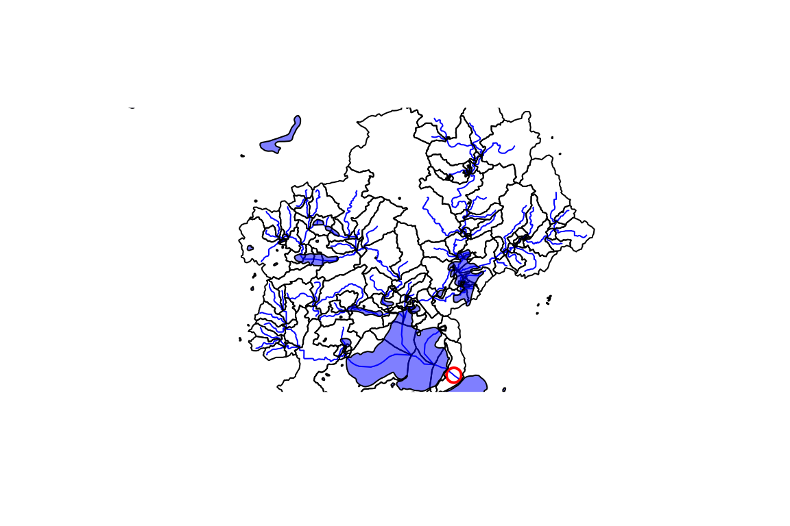
Or fetch NWIS an site as the starting point and generate a plot. Data is returned and/or stored in a local file for later use.
# ?plot_nhdplus for more
plot_data <- plot_nhdplus(
  outlets = list(featureSource = "nwissite", featureID = "USGS-05428500"),
  gpkg = subset_file, overwrite = TRUE)
#> Spherical geometry (s2) switched off
#> although coordinates are longitude/latitude, st_intersects assumes that they
#> are planar
#> Spherical geometry (s2) switched on
#> Zoom set to: 11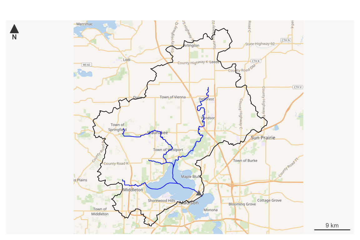
This vignette covers a range of utilities the nhdplusTools package offers for working with data in a U.S. context.
The first thing you are going to need to do is go get some data to
work with. nhdplusTools provides the ability to download
small subsets of the NHDPlus directly from web services. For large
subsets, greater than a few thousand square kilometers, you can use
download_nhdplusv2().
If you are working with the whole National Seamless database,
nhdplusTools has some convenience functions you should be
aware of. Once you have it downloaded and extracted, you can tell the
nhdplusTools package where it is with the nhdplus_path()
function.
nhdplus_path(file.path(work_dir, "natseamless.gpkg"))

basename(nhdplus_path())
#> [1] "natseamless.gpkg"
If you are going to be loading and reloading the flowlines, flowline
attributes, or catchments, repeatedly, the
stage_national_data() function will speed things up a bit.
It creates three staged files that are quicker for R to read at the path
you tell it. If you call it and its output files exist, it won’t
overwrite and just return the paths to your staged files.
staged_data <- stage_national_data(output_path = tempdir())

str(lapply(staged_data, basename))
#> List of 3
#>  $ attributes: chr "nhdplus_flowline_attributes.rds"
#>  $ flowline  : chr "nhdplus_flowline.rds"
#>  $ catchment : chr "nhdplus_catchment.rds"
stage_national_data() assumes you want to stage data in
the same folder as the nhdplus_path database and returns a list of .rds
files that can be read with readRDS. The flowlines and catchments are sf
data.frames and attributes is a plain
data.frame with the attributes from flowline.
Note that this introduction uses a small subset of the national seamless
database as shown in the plot.
flowline <- readRDS(staged_data$flowline)
names(flowline)[1:10]
#>  [1] "COMID"      "FDATE"      "RESOLUTION" "GNIS_ID"    "GNIS_NAME"
#>  [6] "LENGTHKM"   "REACHCODE"  "FLOWDIR"    "WBAREACOMI" "FTYPE"

library(sf)
plot(sf::st_geometry(flowline))
If you don’t need or want all the geometry for the flowlines,
consider using get_vaa(). It allows you to retrieve
specific NHDPlus attributes with very little overhead. It also supports
access to an updated set of network attributes that incorporate numerous
network updates from national hydrologic modelling projects.
vaa <- get_vaa()
names(vaa)
#>  [1] "comid"      "streamleve" "streamorde" "streamcalc" "fromnode"
#>  [6] "tonode"     "hydroseq"   "levelpathi" "pathlength" "terminalpa"
#> [11] "arbolatesu" "divergence" "startflag"  "terminalfl" "dnlevel"
#> [16] "thinnercod" "uplevelpat" "uphydroseq" "dnlevelpat" "dnminorhyd"
#> [21] "dndraincou" "dnhydroseq" "frommeas"   "tomeas"     "reachcode"
#> [26] "lengthkm"   "fcode"      "vpuin"      "vpuout"     "areasqkm"
#> [31] "totdasqkm"  "divdasqkm"  "totma"      "wbareatype" "pathtimema"
#> [36] "slope"      "slopelenkm" "ftype"      "gnis_name"  "gnis_id"
#> [41] "wbareacomi" "hwnodesqkm" "rpuid"      "vpuid"      "roughness"
nrow(vaa)
#> [1] 2691339
NHDPlus HiRes
NHDPlus HiRes is an in-development dataset that introduces much more
dense flowlines and catchments. In the long run,
nhdplusTools will have complete support for NHDPlus HiRes.
So far, nhdplusTools will help download and interface
NHDPlus HiRes data with existing nhdplusTools
functionality. It’s important to note that nhdplusTools was
primarily implemented using NHDPlusV2 and any use of HiRes should be
subject to scrutiny.
For the demo below, a small sample of HiRes data that has been loaded
into nhdplusTools is used. The first line shows how you can
download additional data (just change download_files to
TRUE).
download_nhdplushr(nhd_dir = "download_dir",
                   hu_list = c("0101"), # can mix hu02 and hu04 codes.
                   download_files = FALSE) # TRUE will download files.
#> [1] "https://prd-tnm.s3.amazonaws.com/StagedProducts/Hydrography/NHDPlusHR/Beta/GDB/NHDPLUS_H_0101_HU4_GDB.zip"

out_gpkg <- file.path(work_dir, "nhd_hr.gpkg")
hr_data <- get_nhdplushr(work_dir,
                         out_gpkg = out_gpkg)
(layers <- st_layers(out_gpkg))
#> Driver: GPKG
#> Available layers:
#>         layer_name geometry_type features fields             crs_name
#> 1      NHDFlowline   Line String     2691     57 GRS 1980(IUGG, 1980)
#> 2 NHDPlusCatchment Multi Polygon     2603      7 GRS 1980(IUGG, 1980)
#> 3     NHDWaterbody       Polygon     1044     15 GRS 1980(IUGG, 1980)
#> 4          NHDArea       Polygon       10     14 GRS 1980(IUGG, 1980)
#> 5          NHDLine   Line String      142     12 GRS 1980(IUGG, 1980)
#> 6      NHDPlusSink         Point        1     10 GRS 1980(IUGG, 1980)
#> 7         NHDPoint      3D Point        7     10 GRS 1980(IUGG, 1980)
names(hr_data)
#> [1] "NHDFlowline"      "NHDPlusCatchment"
unlink(out_gpkg)

hr_data <- get_nhdplushr(work_dir,
                         out_gpkg = out_gpkg,
                         layers = NULL)
<<<<<<< HEAD
#> defaulting to comid rather than permanent_identifier
=======
>>>>>>> main
(layers <- st_layers(out_gpkg))
#> Driver: GPKG
#> Available layers:
#>         layer_name geometry_type features fields             crs_name
#> 1      NHDFlowline   Line String     2691     57 GRS 1980(IUGG, 1980)
#> 2 NHDPlusCatchment Multi Polygon     2603      7 GRS 1980(IUGG, 1980)
#> 3     NHDWaterbody       Polygon     1044     15 GRS 1980(IUGG, 1980)
#> 4          NHDArea       Polygon       10     14 GRS 1980(IUGG, 1980)
#> 5          NHDLine   Line String      142     12 GRS 1980(IUGG, 1980)
#> 6      NHDPlusSink         Point        1     10 GRS 1980(IUGG, 1980)
#> 7         NHDPoint      3D Point        7     10 GRS 1980(IUGG, 1980)
names(hr_data)
#> [1] "NHDFlowline"      "NHDPlusCatchment" "NHDWaterbody"     "NHDArea"
#> [5] "NHDLine"          "NHDPlusSink"      "NHDPoint"
Discovery and Subsetting
One of the primary workflows nhdplusTools is designed to
accomplish can be described in three steps:
- what NHDPlus catchment is at the outlet of a watershed,
- figure out what catchments are up or downstream of that catchment, and
- create a stand alone subset for that collection of catchments.
Say we want to get a subset of the NHDPlus upstream of a given
location. We can start with discover_nhdplus_id() First,
let’s look at a given point location. Then see where it is relative to
our flowlines.
lon <- -89.36
lat <- 43.09

start_point <- sf::st_sfc(sf::st_point(c(lon, lat)),
                          crs = 4269)

plot(sf::st_geometry(flowline))
plot(start_point, cex = 1.5, lwd = 2, col = "red", add = TRUE)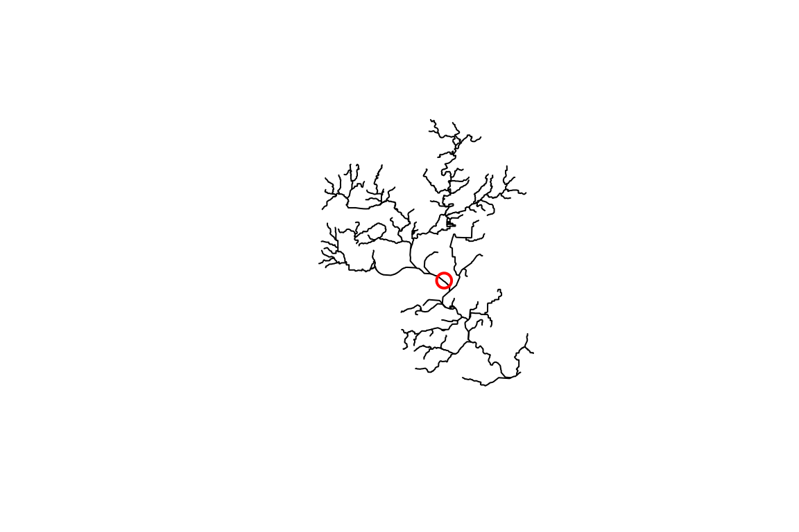
OK, so we have a point location near a river and we want to figure
out what catchment is at its outlet. We can use the
discover_nhdplus_id() function which calls out to a web
service and returns an NHDPlus catchment identifier, typically called a
COMID.
If we set raindrop = TRUE, we can also get a elevation
derived downslope trace to the nearest flowline and some additional
info. See get_raindrop_trace() for more on this
functionality.
start_comid <- discover_nhdplus_id(start_point, raindrop = TRUE)
start_comid
#> Simple feature collection with 2 features and 7 fields
#> Geometry type: LINESTRING
#> Dimension:     XY
#> Bounding box:  xmin: -89.37037 ymin: 43.08522 xmax: -89.35393 ymax: 43.09491
#> Geodetic CRS:  WGS 84
#> # A tibble: 2 × 8
#>   id    gnis_name   comid reachcode raindrop_pathDist measure intersection_point
#>   <chr> <chr>       <int> <chr>                 <dbl>   <dbl> <list>
#> 1 nhdF… Yahara R…  1.33e7 07090002…              124.    40.1 <dbl [2]>
#> 2 rain… NA        NA      NA                      NA     NA   <dbl [0]>
#> # ℹ 1 more variable: geometry <LINESTRING [°]>

plot(sf::st_geometry(start_comid))
plot(sf::st_geometry(flowline), add = TRUE, col = "blue", lwd = 2)
plot(start_point, cex = 1.5, lwd = 2, col = "red", add = TRUE)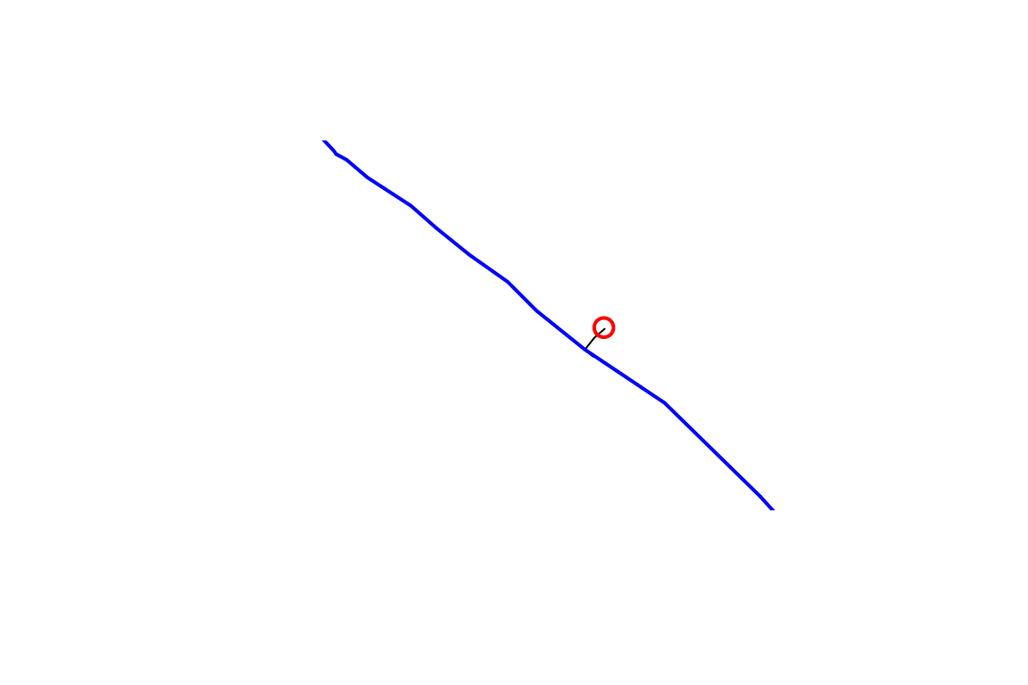
If you have the whole National Seamless database and want to work at regional to national scales, skip down the the Local Data Subsetting section.
Web Service Data Subsetting
nhdplusTools supports discovery and data subsetting
using web services made available through the Network Linked Data
Index (NLDI) and the National Water Census
Geoserver. The code below shows how to use the NLDI functions to
build a dataset upstream of our start_comid that we found
above.
The NLDI can be queried with any set of watershed outlet locations that it has in its index. We call these “featureSources”. We can query the NLDI for an identifier of a given feature from any of its “featureSources” and find out what our navigation options are as shown below.
dataRetrieval::get_nldi_sources()$source
<<<<<<< HEAD
#>  [1] "ca_gages"       "epa_nrsa"       "geoconnex-demo" "gfv11_pois"
#>  [5] "huc12pp"        "nmwdi-st"       "nwisgw"         "nwissite"
#>  [9] "ref_gage"       "vigil"          "wade"           "WQP"
#> [13] "comid"
=======
#>  [1] "ca_gages"          "census2020-nhdpv2" "epa_nrsa"
#>  [4] "geoconnex-demo"    "gfv11_pois"        "huc12pp"
#>  [7] "nmwdi-st"          "npdes"             "nwisgw"
#> [10] "nwissite"          "ref_gage"          "vigil"
#> [13] "wade"              "WQP"               "comid"
>>>>>>> main

nldi_feature <- list(featureSource = "comid",
                     featureID = as.integer(start_comid$comid)[1])

get_nldi_feature(nldi_feature)
#> Simple feature collection with 1 feature and 3 fields
#> Geometry type: LINESTRING
#> Dimension:     XY
#> Bounding box:  xmin: -89.37037 ymin: 43.08521 xmax: -89.35393 ymax: 43.09491
#> Geodetic CRS:  WGS 84
#> # A tibble: 1 × 4
#>   sourceName    identifier comid                                        geometry
#>   <chr>         <chr>      <chr>                                <LINESTRING [°]>
#> 1 NHDPlus comid 13293750   13293750 (-89.37037 43.09491, -89.36997 43.09475, -8…
We can use get_nldi_feature() as a way to make sure the
featureID is available for the chosen “featureSource”. Now that we know
the NLDI has our comid, we can use the “upstreamTributaries” navigation
option to get all the flowlines upstream or all the features from any of
the “featureSources” as shown below.
flowline_nldi <- navigate_nldi(nldi_feature,
                               mode = "upstreamTributaries",
                               distance_km = 1000)

plot(sf::st_geometry(flowline), lwd = 3, col = "black")
plot(sf::st_geometry(flowline_nldi$origin), lwd = 3, col = "red", add = TRUE)
plot(sf::st_geometry(flowline_nldi$UT), lwd = 1, col = "red", add = TRUE)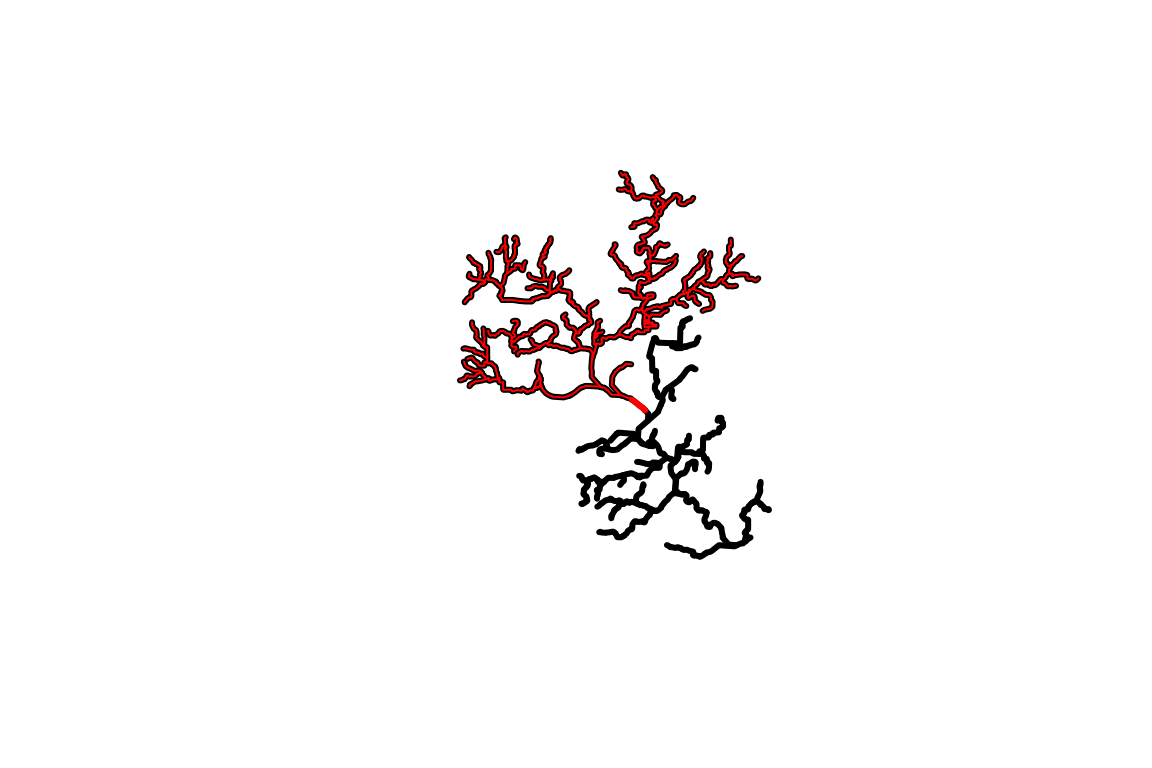
The NLDI only provides geometry and a comid for each of the
flowlines. The subset_nhdplus() function has a “download”
option that allows us to download four layers and all attributes as
shown below. There is also a navigate_network() function
that will replace navigate_nldi() and
subset_nhdplus() for many use cases.
output_file_download <- file.path(work_dir, "subset_download.gpkg")

output_file_download <-subset_nhdplus(comids = as.integer(flowline_nldi$UT$nhdplus_comid),
                                      output_file = output_file_download,
                                      nhdplus_data = "download", return_data = FALSE,
                                      overwrite = TRUE)
#> All intersections performed in latitude/longitude.
#> Reading NHDFlowline_Network
#> Spherical geometry (s2) switched off
#> Spherical geometry (s2) switched on
#> Writing NHDFlowline_Network

sf::st_layers(output_file_download)
#> Driver: GPKG
#> Available layers:
#>            layer_name geometry_type features fields crs_name
#> 1 NHDFlowline_Network   Line String      168    137    NAD83

flowline_download <- sf::read_sf(file.path(work_dir, "subset_download.gpkg"),
                                 "NHDFlowline_Network")

plot(sf::st_geometry(dplyr::filter(flowline_download,
                                   streamorde > 2)),
     lwd = 7, col = "darkgrey")
plot(sf::st_geometry(flowline_nldi$UT),
     lwd = 3, col = "red", add = TRUE)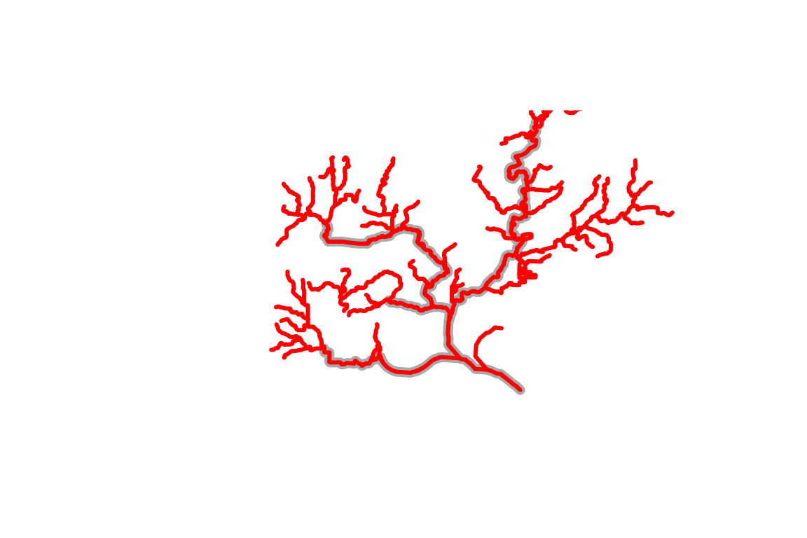
This plot illustrates the kind of thing that’s possible (filtering to specific stream orders) using the attributes that are downloaded.
Before moving on, one more demonstration of what can be done using the NLDI. Say we knew the USGS gage ID that we want NHDPlus data upstream of. We can use the NLDI to navigate from the gage the same as we did for our comid. We can also get back all the nwis sites the NLDI knows about upstream of the one we chose!
nldi_feature <- list(featureSource = "nwissite",
                     featureID = "USGS-05428500")

flowline_nldi <- navigate_nldi(nldi_feature,
                               mode = "upstreamTributaries",
                               distance_km = 1000)

output_file_nwis <- file.path(work_dir, "subset_download_nwis.gpkg")

output_file_nwis <-subset_nhdplus(comids = as.integer(flowline_nldi$UT$nhdplus_comid),
                                  output_file = output_file_nwis,
                                  nhdplus_data = "download",
                                  return_data = FALSE, overwrite = TRUE)
#> All intersections performed in latitude/longitude.
#> Reading NHDFlowline_Network
#> Spherical geometry (s2) switched off
#> Spherical geometry (s2) switched on
#> Writing NHDFlowline_Network

sf::st_layers(output_file_download)
#> Driver: GPKG
#> Available layers:
#>            layer_name geometry_type features fields crs_name
#> 1 NHDFlowline_Network   Line String      168    137    NAD83

flowline_nwis <- sf::read_sf(output_file_nwis,
                                 "NHDFlowline_Network")

upstream_nwis <- navigate_nldi(nldi_feature,
                               mode = "upstreamTributaries",
                               data_source = "nwissite",
                               distance_km = 1000)

plot(sf::st_geometry(flowline_nwis),
     lwd = 3, col = "blue")
plot(sf::st_geometry(upstream_nwis$UT_nwissite),
     cex = 1, lwd = 2, col = "red", add = TRUE)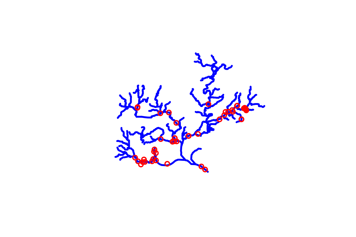
Local Data Subsetting
While web service data access is very convenient, some use cases make working with web services impossible or cumbersome such that working with local data is preferable. nhdplusTools supports such workflows with hybrid, web-service and local, workflows.
With the starting COMID we found with
discover_nhdplus_id() above, we can use one of the network
navigation functions, get_UM(), get_UT(),
get_DM(), or get_DD() to retrieve a collection
of comids along the upstream mainstem, upstream with tributaries,
downstream mainstem, or downstream with diversions network paths. Here
we’ll use upstream with tributaries.
UT_comids <- get_UT(flowline, start_comid$comid[1])
UT_comids
#>   [1]  13293750  13293504  13294134  13294128  13294394  13293454  13293430
#>   [8]  13293424  13294110  13293398  13293392  13293388  13293384  13293380
#>  [15]  13293576  13294288  13294284  13293506  13294280  13294290  13294298
#>  [22]  13294304  13294310  13294312  13293696  13293694  13294264  13293676
#>  [29]  13293620  13293612  13293584  13294166  13293554  13293540  13294282
#>  [36]  13293520  13293480  13294132  13293588  13293550  13293574  13293508
#>  [43]  13293530  13293526  13293524  13294138  13293496  13293488  13293484
#>  [50]  13293474  13294118  13293440  13293426  13293458  13294382  13294274
#>  [57]  13293422  13293416  13293390  13293382  13293386  13293376  13293396
#>  [64]  13293394  13293406  13293404  13294268  13294366  13293400  13293432
#>  [71]  13293452  13293456  13293492  13294158  13294286  13293634  13294368
#>  [78]  13294124 937090090 937090091  13293464  13293444  13293446  13293434
#>  [85]  13293542  13294154  13293536  13294292  13294294  13294300  13294308
#>  [92]  13294314  13294272  13294276  13294384  13294278  13294386  13293494
#>  [99]  13294130  13294306  13294184  13293690  13293692  13293586  13293614
#> [106]  13293624  13293678  13293672  13293674  13294176  13294168  13293578
#> [113]  13293564  13293548  13293478  13293476  13293450  13293442  13293518
#> [120]  13293472  13293572  13293568  13293556  13293558  13293552  13293514
#> [127]  13293522  13294144  13293532  13294150  13294148  13294140  13293516
#> [134]  13293502  13293498  13293460  13294122  13293468  13294112  13293512
#> [141]  13293486  13293378  13293462  13293428  13293420  13293412  13293438
#> [148]  13293490  13293436  13294152  13294296  13294270  13302588  13302590
#> [155]  13293688  13293646  13294174  13294178  13293562  13293600  13293448
#> [162]  13294116  13294120  13293570  13294114  13293418  13293410  13293590
If you are familiar with the NHDPlus, you will recognize that now
that we have this list of COMIDs, we could go off and do all sorts of
things with the various flowline attributes. For now, let’s just use the
COMID list to filter our fline sf
data.frame and plot it with our other layers.
plot(sf::st_geometry(flowline))
plot(start_point, cex = 1.5, lwd = 2, col = "red", add = TRUE)
plot(sf::st_geometry(dplyr::filter(flowline, COMID %in% UT_comids)),
     add=TRUE, col = "red", lwd = 2)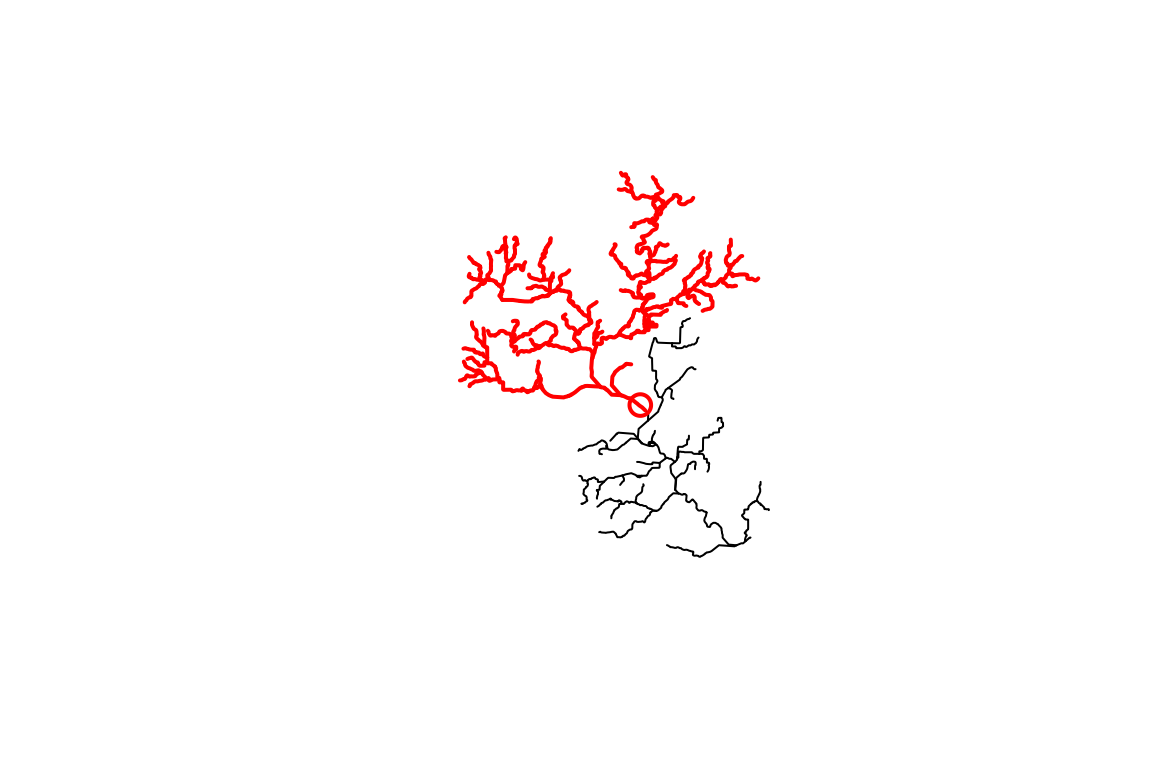
Say you want to save the network subset for later use in R or in some
other GIS. The subset_nhdplus() function is your friend. If
you have the whole national seamless database downloaded, you can pull
out large subsets of it like shown below (this queries for data from the
local geodatabase without loading the whole thing into memory). If you
don’t have the whole national seamless, look at the second example in
this section.
output_file <- file.path(work_dir, "subset.gpkg")

output_file <-subset_nhdplus(comids = UT_comids,
                             output_file = output_file,
                             nhdplus_data = nhdplus_path(),
                             return_data = FALSE, overwrite = TRUE)
#> All intersections performed in latitude/longitude.
#> Reading NHDFlowline_Network
#> 168 comids of 168
#> Writing NHDFlowline_Network
#> Reading CatchmentSP
#> 168 comids of 168
#> Writing CatchmentSP
#> Reading NHDArea
#> Writing NHDArea
#> Reading NHDWaterbody
#> Writing NHDWaterbody
#> Reading NHDFlowline_NonNetwork
#> Writing NHDFlowline_NonNetwork
#> Reading Gage
#> Writing Gage
#> Reading Sink
#> No features to write in Sink

sf::st_layers(output_file)
#> Driver: GPKG
#> Available layers:
#>               layer_name geometry_type features fields crs_name
#> 1    NHDFlowline_Network   Line String      168    136    NAD83
#> 2            CatchmentSP Multi Polygon      167      6    NAD83
#> 3                NHDArea       Polygon        1     14    NAD83
#> 4           NHDWaterbody       Polygon       90     21    NAD83
#> 5 NHDFlowline_NonNetwork   Line String       45     12    NAD83
#> 6                   Gage         Point       33     19    NAD83
Now we have an output geopackage that can be used later. It contains the network subset of catchments and flowlines as well as a spatial subset of other layers as shown in the status output above. To complete the demonstration, here are a couple more layers plotted up.
catchment <- sf::read_sf(output_file, "CatchmentSP")
waterbody <- sf::read_sf(output_file, "NHDWaterbody")

plot(sf::st_geometry(flowline))
plot(start_point, cex = 1.5, lwd = 2, col = "red", add = TRUE)
plot(sf::st_geometry(dplyr::filter(flowline, COMID %in% UT_comids)),
     add=TRUE, col = "red", lwd = 2)
plot(sf::st_geometry(catchment), add = TRUE)
plot(sf::st_geometry(waterbody), col = rgb(0, 0, 1, alpha = 0.5), add = TRUE)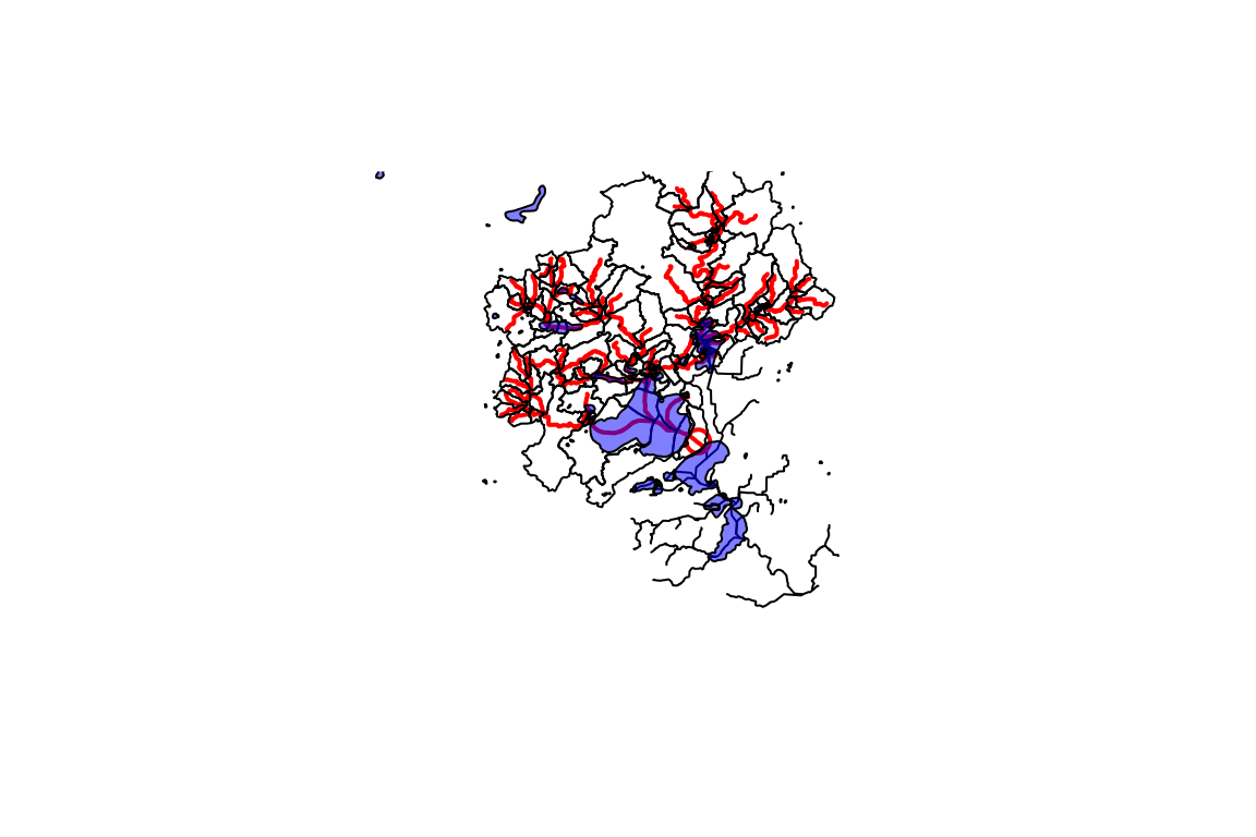
Indexing
nhdplusTools supports a number of indexing use cases. See the function index for specifics.
Using the data above, we can use the
get_flowline_index() function to get the comid, reachcode,
and measure of our starting point like this.
get_flowline_index(flowline, start_point)
<<<<<<< HEAD
#> Warning in match_crs(x, points, paste("crs of lines and points don't match.", :
#> crs of lines and points don't match. attempting st_transform of lines
#> Warning in index_points_to_lines.hy(x, points, search_radius = search_radius, :
#> converting to LINESTRING, this may be slow, check results
=======
#> Warning in match_crs(flines, points, paste("crs of lines and points don't
#> match.", : crs of lines and points don't match. attempting st_transform of
#> lines
>>>>>>> main
#>   id    COMID      REACHCODE REACH_meas       offset
#> 1  1 13293750 07090002007373    41.8003 0.0009621378
get_flowline_index() will work with a list of points
too. For demonstration purposes, we can use the gages in our subset from
above.
gage <- sf::read_sf(output_file, "Gage")

get_flowline_index(flowline, sf::st_geometry(gage), precision = 10)
<<<<<<< HEAD
#> Warning in match_crs(x, points, paste("crs of lines and points don't match.", :
#> crs of lines and points don't match. attempting st_transform of lines
=======
#> Warning in match_crs(flines, points, paste("crs of lines and points don't
#> match.", : crs of lines and points don't match. attempting st_transform of
#> lines
>>>>>>> main
#>    id    COMID      REACHCODE REACH_meas         offset
#> 1   1 13293744 07090002007743    29.3045 0.000016031339
#> 2   2 13294276 07090002008387    50.4424 0.000012319388
#> 3   3 13294264 07090002007650    13.4601 0.000020924187
#> 4   4 13293750 07090002007373    10.6795 0.000025343524
#> 5   5 13294312 07090002008383     1.3256 0.000002976034
#> 6   6 13294264 07090002007650    53.7358 0.000033122595
#> 7   7 13294264 07090002007650     6.9114 0.000002256005
#> 8   9 13294300 07090002008379    71.0369 0.000016082151
#> 9  10 13293690 07090002007648     0.7642 0.000014026098
#> 10 11 13294264 07090002007650     8.4036 0.008204857099
#> 11 13 13294176 07090002007664    12.0361 0.000031905454
#> 12 15 13294290 07090002008374    88.0213 0.000027985042
#> 13 16 13294138 07090002007709    54.6248 0.000010977009
#> 14 18 13293486 07090002007724    28.9826 0.000012426106
#> 15 19 13293512 07090002007723    67.1840 0.000010481501
#> 16 20 13294176 07090002007664    42.3100 0.000012406860
#> 17 22 13293474 07090002007713    66.1583 0.000006053102
#> 18 23 13293520 07090002007676    45.5538 0.000030263717
#> 19 24 13293876 07090002007627    54.6477 0.000025453648
#> 20 25 13294374 07090002007633    46.8761 0.000002619625
#> 21 26 13293512 07090002007723    49.3024 0.000025778329
#> 22 27 13294264 07090002007650    90.8928 0.000013950790
#> 23 28 13294344 07090002007629    12.2123 0.000007648685
#> 24 29 13293456 07090002007738    90.8364 0.000036283275
#> 25 30 13294344 07090002007629    51.4760 0.000012934585
#> 26 31 13293512 07090002007723    47.7360 0.000022459225
#> 27 32 13294344 07090002007629    12.2123 0.000007648685
#> 28 33 13293576 07090002008236     2.7112 0.000009945223
For more info about get_flowline_index() and other
indexing functions, see the article vignette("indexing")
about it or the reference page that describes it.