09: GeoPandas - DataFrames with geometry for GIS applications
[1]:
import os
import numpy as np
import pandas as pd
import geopandas as gp
from pathlib import Path
from shapely.geometry import Point, Polygon
[2]:
datapath = Path('data/geopandas/')
Nice overview tutorial Examples Gallery
OVERVIEW
In this notebook we will explore how geopandas works with GIS data (e.g. shapefiles and the objects within them) using geometrically-aware DataFrames. We will also explore how common GIS-related operations are available in geopandas. This notebook relies on publicly available GIS datasets for the city of Madison, Wisconsin.
get some data - read_file is the ticket for GeoJSON, shapefiles, GDB, etc.
[3]:
parks = gp.read_file(datapath / 'Madison_Parks.geojson')
writing back out is veeeery similar with to_file but give a few options for formats
[4]:
parks.to_file(datapath / "parks.shp")
/tmp/ipykernel_6596/3998401397.py:1: UserWarning: Column names longer than 10 characters will be truncated when saved to ESRI Shapefile.
  parks.to_file(datapath / "parks.shp")
/home/runner/micromamba/envs/pyclass-docs/lib/python3.14/site-packages/pyogrio/raw.py:733: RuntimeWarning: Normalized/laundered field name: 'SHAPESTArea' to 'SHAPESTAre'
  ogr_write(
/home/runner/micromamba/envs/pyclass-docs/lib/python3.14/site-packages/pyogrio/raw.py:733: RuntimeWarning: Normalized/laundered field name: 'SHAPESTLength' to 'SHAPESTLen'
  ogr_write(
[5]:
# or with a different driver
parks.to_file(datapath / "parks.json", driver='GeoJSON')
this now looks like a Pandas DataFrame but there’s a special column geometry
[6]:
parks.head()
[6]:
| OBJECTID | Park_ID | Type | Acreage | Park_Name | ShortName | Subtype | SHAPESTArea | SHAPESTLength | geometry | |
|---|---|---|---|---|---|---|---|---|---|---|
| 0 | 6416 | 3120 | MINI | 7.72 | Quarry Cove Park | Quarry Cove | NaN | 3.363779e+05 | 2808.992197 | POLYGON ((-89.48419 43.00851, -89.48416 43.010... |
| 1 | 6417 | 2610 | MINI | 2.36 | Sunridge Park | Sunridge | NaN | 1.027629e+05 | 1284.462030 | POLYGON ((-89.48162 43.04065, -89.4816 43.0410... |
| 2 | 6418 | 3320 | MINI | 1.09 | Lederberg Park | Lederberg | NaN | 4.752503e+04 | 940.774563 | POLYGON ((-89.53472 43.05151, -89.53511 43.052... |
| 3 | 6419 | 3020 | MINI | 3.22 | Village Park | Village | NaN | 1.402491e+05 | 1779.319445 | POLYGON ((-89.28712 43.16125, -89.28711 43.161... |
| 4 | 6420 | 1500 | COMMUNITY | 51.02 | Olin Park | Olin | NaN | 2.222246e+06 | 12658.852710 | MULTIPOLYGON (((-89.3763 43.05509, -89.37636 4... |
also some important metadata particularly the CRS
[7]:
parks.crs
[7]:
<Geographic 2D CRS: EPSG:4326>
Name: WGS 84
Axis Info [ellipsoidal]:
- Lat[north]: Geodetic latitude (degree)
- Lon[east]: Geodetic longitude (degree)
Area of Use:
- name: World.
- bounds: (-180.0, -90.0, 180.0, 90.0)
Datum: World Geodetic System 1984 ensemble
- Ellipsoid: WGS 84
- Prime Meridian: Greenwich
pro tip: You can have multiple geometry columns but only one is active – this is important later as we do operations on GeoDataFrames. The column labeled
geometryis typically the active one but you you can change it.
So what’s up with these geometries? They are represented as `shapely <https://shapely.readthedocs.io/en/stable/manual.html>`__ objects so can be:
polygon / multi-polygon
point / multi-point
line / multi-line
we can access with pandas loc and iloc references
[8]:
parks.iloc[1].geometry.geom_type
[8]:
'Polygon'
[9]:
parks.loc[parks.ShortName=='Olin'].geometry.geom_type
[9]:
4    MultiPolygon
dtype: str
There are other cool shapely properties like area
[10]:
parks.loc[parks.ShortName=='Olin'].geometry.area
/tmp/ipykernel_6596/2331563363.py:1: UserWarning: Geometry is in a geographic CRS. Results from 'area' are likely incorrect. Use 'GeoSeries.to_crs()' to re-project geometries to a projected CRS before this operation.

  parks.loc[parks.ShortName=='Olin'].geometry.area
[10]:
4    0.000023
dtype: float64
ruh-roh - what’s up with this CRS and tiny area number?
[11]:
parks.crs
[11]:
<Geographic 2D CRS: EPSG:4326>
Name: WGS 84
Axis Info [ellipsoidal]:
- Lat[north]: Geodetic latitude (degree)
- Lon[east]: Geodetic longitude (degree)
Area of Use:
- name: World.
- bounds: (-180.0, -90.0, 180.0, 90.0)
Datum: World Geodetic System 1984 ensemble
- Ellipsoid: WGS 84
- Prime Meridian: Greenwich
area units in lat/long don’t make sense. Let’s project to something in meters (but how?) to_crs will do it, but importantly, either reassign or set inplace=True
[12]:
parks.to_crs(3071, inplace=True)
parks.crs
[12]:
<Projected CRS: EPSG:3071>
Name: NAD83(HARN) / Wisconsin Transverse Mercator
Axis Info [cartesian]:
- X[east]: Easting (metre)
- Y[north]: Northing (metre)
Area of Use:
- name: United States (USA) - Wisconsin.
- bounds: (-92.89, 42.48, -86.25, 47.31)
Coordinate Operation:
- name: Wisconsin Transverse Mercator 83
- method: Transverse Mercator
Datum: NAD83 (High Accuracy Reference Network)
- Ellipsoid: GRS 1980
- Prime Meridian: Greenwich
[13]:
parks.loc[parks.ShortName=='Olin'].geometry.area
[13]:
4    206286.146769
dtype: float64
there are loads of useful methods for shapely objects for relationships between geometries (intersection, distance, etc.) but we will skip these for now because GeoPandas facilitates these things for entire geodataframes! #sick
Pro Tip: There are occasions when, while connected to VPN, the first geometry in a GeoGataDrame has its CRS set to infinity rather than a target CRS. There are a couple potential fixes for that here
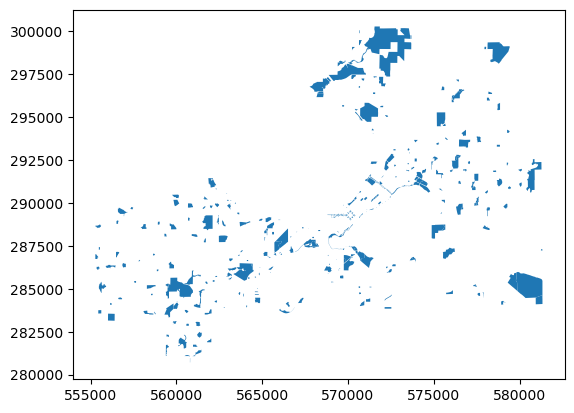
So back to GeoDataFrames…..we can look at them spatially as well with plot()
[14]:
parks.plot()
[14]:
<Axes: >
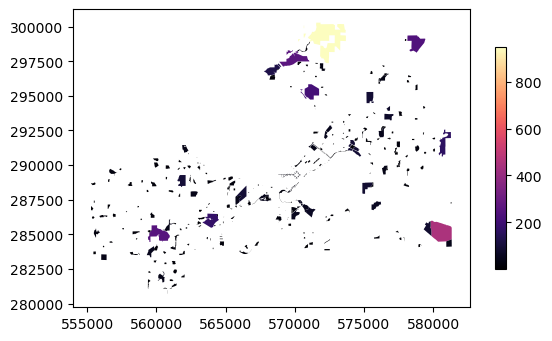
easily make a chloropleth map using a selected column as the color (and add a legend) using plot()
[15]:
parks.columns
[15]:
Index(['OBJECTID', 'Park_ID', 'Type', 'Acreage', 'Park_Name', 'ShortName',
       'Subtype', 'SHAPESTArea', 'SHAPESTLength', 'geometry'],
      dtype='str')
[16]:
parks.sample(4)
[16]:
| OBJECTID | Park_ID | Type | Acreage | Park_Name | ShortName | Subtype | SHAPESTArea | SHAPESTLength | geometry | |
|---|---|---|---|---|---|---|---|---|---|---|
| 211 | 6631 | 1582 | NEIGHBORHOOD | 12.79 | Odana Hills Park | Odana Hills | NaN | 556909.477173 | 4101.074463 | POLYGON ((563041.29 286112.105, 563054.556 286... |
| 178 | 6596 | 2341 | CONSERVATION | 11.78 | Hiestand Woods | Hiestand | NaN | 513028.051300 | 4608.909910 | POLYGON ((576370.636 292700.346, 576465.947 29... |
| 250 | 6670 | 2590 | MINI | 0.37 | Peace (Elizabeth Link) Park | Peace | NaN | 14871.681427 | 539.883865 | POLYGON ((569429.405 289312.699, 569450.13 289... |
| 225 | 6645 | 2301 | CONSERVATION | 5.28 | Paunack (A.O.) Marsh | Paunack | NaN | 229917.956512 | 2091.617871 | POLYGON ((573805.377 286693.694, 573943.906 28... |
[17]:
parks.plot(column="Acreage", cmap = 'magma', k=5, legend=True, legend_kwds={'shrink': 0.6})
[17]:
<Axes: >
also a very cool interactive plot options with a basemap using explore()
[18]:
parks.explore(column='Acreage', cmap='magma')
[18]:
we can read in another shapefile
[19]:
hoods = gp.read_file(datapath / 'Neighborhood_Associations.geojson')
[20]:
hoods.sample(5)
[20]:
| OBJECTID | NA_ID | NEIGHB_NAME | STATUS | CLASSIFICA | Web | ShapeSTArea | ShapeSTLength | geometry | |
|---|---|---|---|---|---|---|---|---|---|
| 90 | 9937 | 126 | Park Ridge Neighborhood Association | Inactive | Neighborhood Association | http://www.cityofmadison.com/neighborhoods/pro... | 1.319349e+06 | 4997.382801 | POLYGON ((-89.50231 43.0404, -89.50221 43.0404... |
| 108 | 9955 | 160 | Twin Oaks Neighborhood Association | Active | Neighborhood Association | http://www.cityofmadison.com/neighborhoods/pro... | 1.141939e+06 | 5417.482020 | POLYGON ((-89.28913 43.03144, -89.28913 43.031... |
| 63 | 9910 | 84 | Skyview Meadows Neighborhood Association | Inactive | Neighborhood Association | http://www.cityofmadison.com/neighborhoods/pro... | 4.081868e+06 | 10648.841043 | POLYGON ((-89.50718 43.03038, -89.50718 43.030... |
| 88 | 9935 | 121 | Prairie Hills Neighborhood Association | Active | Neighborhood Association | http://www.cityofmadison.com/neighborhoods/pro... | 1.449706e+07 | 19445.385990 | POLYGON ((-89.48725 43.03633, -89.48694 43.036... |
| 18 | 9865 | 22 | East Bluff Homeowners Association | Active | Condominium Association | http://www.cityofmadison.com/neighborhoods/pro... | 6.502308e+05 | 3345.493777 | POLYGON ((-89.3635 43.1312, -89.36347 43.13194... |
and we can plot these on top of each other
[21]:
ax_hood = hoods.plot()
# now plot the other one but specify which axis to plot on (ax=ax_hood)
parks.plot(column="Acreage", cmap = 'magma', k=5, legend=True, legend_kwds={'shrink': 0.6}, ax=ax_hood)
[21]:
<Axes: >
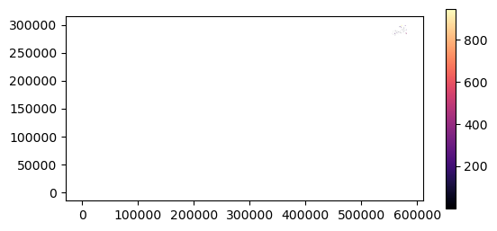
WAT! Why so far apart?
[22]:
hoods.crs
[22]:
<Geographic 2D CRS: EPSG:4326>
Name: WGS 84
Axis Info [ellipsoidal]:
- Lat[north]: Geodetic latitude (degree)
- Lon[east]: Geodetic longitude (degree)
Area of Use:
- name: World.
- bounds: (-180.0, -90.0, 180.0, 90.0)
Datum: World Geodetic System 1984 ensemble
- Ellipsoid: WGS 84
- Prime Meridian: Greenwich
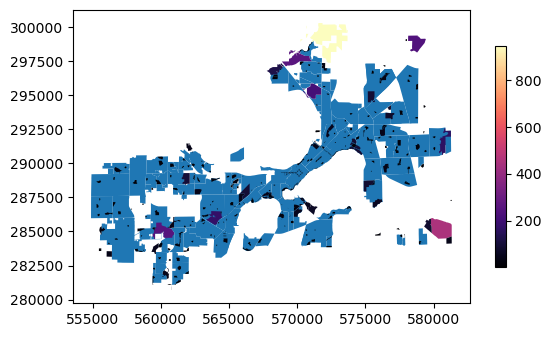
we need to reproject. Geopandas uses to_crs() for this purpose
[23]:
# we can reproject, and set hoods to park crs
hoods.to_crs(parks.crs, inplace=True)
[24]:
ax_hood = hoods.plot()
# now plot the other one but specify which axis to plot on (ax=ax_hood)
parks.plot(column="Acreage", cmap = 'magma', k=5, legend=True, legend_kwds={'shrink': 0.6}, ax=ax_hood)
[24]:
<Axes: >
or similarly with the interactive maps
[25]:
m_hood = hoods.explore()
parks.explore(column="Acreage", cmap = 'magma', k=5, legend=True, legend_kwds={'shrink': 0.6}, m=m_hood)
[25]:
we can make a new geodataframe using shapely properties of the geometry - how about centroids?
make a new geodataframe of the parks
add a columns with centroids for each park
plot an interactive window with the park centroids and the neighborhoods
hints:
remember the shapely methods are available for each geometry object (e.g.
centroid())you can loop over the column in a couple different ways
you can define which columns contains the geometry of a geodataframe
you will likely have to define the CRS
[ ]:
[ ]:
[ ]:
[ ]:
Operations on and among geodataframes…do I need to use a GIS program?
Dissolve
[26]:
hoods.dissolve() # note it defaults to filling all the columns with the first value
[26]:
| geometry | OBJECTID | NA_ID | NEIGHB_NAME | STATUS | CLASSIFICA | Web | ShapeSTArea | ShapeSTLength | |
|---|---|---|---|---|---|---|---|---|---|
| 0 | MULTIPOLYGON (((560429.904 281602.442, 560430.... | 9847 | 1 | Allied Dunn's Marsh Neighborhood Association | Active | Neighborhood Association | http://www.cityofmadison.com/neighborhoods/pro... | 1.512568e+07 | 16657.055614 |
[27]:
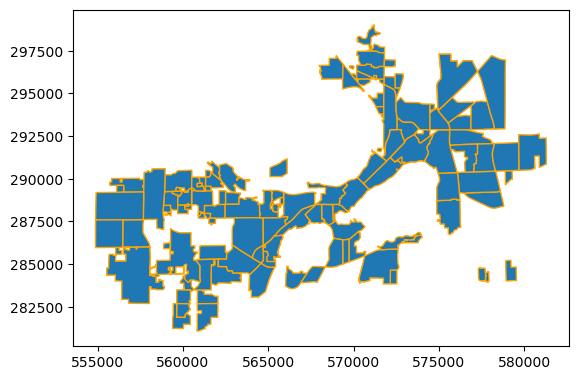
ax=hoods.dissolve().plot()
hoods.plot(facecolor=None, edgecolor='orange', ax=ax)
[27]:
<Axes: >
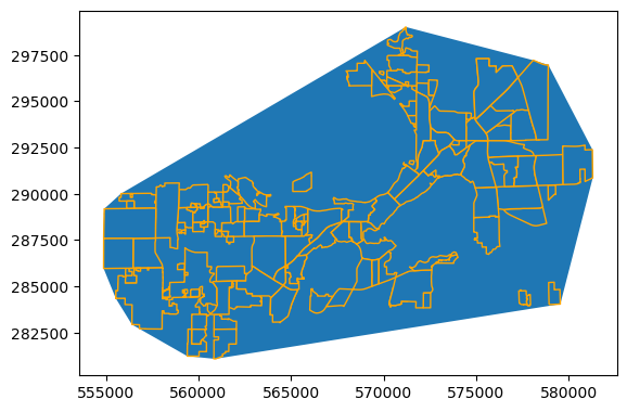
Convex Hull
[28]:
ax = hoods.dissolve().convex_hull.plot()
hoods.plot(facecolor=None, edgecolor='orange', ax=ax)
[28]:
<Axes: >
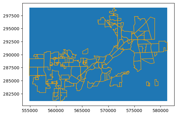
Bounding Box is a little more tricky
[29]:
hoods.bounds # that's per each row
[29]:
| minx | miny | maxx | maxy | |
|---|---|---|---|---|
| 0 | 563872.429544 | 283460.518859 | 565328.837226 | 285057.462675 |
| 1 | 561310.621737 | 289288.751579 | 561646.281647 | 289570.375291 |
| 2 | 566010.016502 | 283558.607236 | 567270.271941 | 284869.636703 |
| 3 | 568527.624082 | 286423.950486 | 570669.728818 | 287657.510073 |
| 4 | 569018.771979 | 288242.314399 | 569250.882412 | 288506.627088 |
| ... | ... | ... | ... | ... |
| 135 | 574180.047766 | 290323.744701 | 576068.029053 | 292858.768636 |
| 136 | 572143.872431 | 290896.914666 | 574663.138190 | 292637.318811 |
| 137 | 554878.971311 | 287588.991000 | 557696.123932 | 289229.663701 |
| 138 | 567269.204147 | 288485.712034 | 569627.785405 | 289802.439174 |
| 139 | 554873.114600 | 285970.029005 | 556474.561414 | 287596.015566 |
140 rows × 4 columns
[30]:
tb = hoods.total_bounds # this gives overall bounds
tb
[30]:
array([554873.11459994, 281085.59466762, 581291.42545321, 299016.88496873])
We can make a polygon from these coordinates with shapely
[31]:
from shapely.geometry import box
[32]:
bbox = box(tb[0], tb[1], tb[2], tb[3])
# pro tip - when passing a bunch of ordered arguments, '*' will unpack them #nice
bbox = box(*hoods.total_bounds)
to make a GeoDataFrame from scratch, the minimum you need is geometry, but a crs is important, and some data will populate more columns
[33]:
hoods_boundary = gp.GeoDataFrame(data={'thing':['bounding_box']},geometry=[bbox], crs=hoods.crs)
hoods_boundary
[33]:
| thing | geometry | |
|---|---|---|
| 0 | bounding_box | POLYGON ((581291.425 281085.595, 581291.425 29... |
[34]:
ax = hoods_boundary.plot()
hoods.plot(facecolor=None, edgecolor='orange', ax=ax)
[34]:
<Axes: >
How about some spatial joins?
we can bring in information based on locational overlap. Let’s look at just a couple neighborhoods (Marquette and Tenny-Lapham) on the Isthmus
[35]:
isthmus = hoods.loc[hoods['NEIGHB_NAME'].str.contains('Marquette') |
                   hoods['NEIGHB_NAME'].str.contains('Tenney')]
isthmus
[35]:
| OBJECTID | NA_ID | NEIGHB_NAME | STATUS | CLASSIFICA | Web | ShapeSTArea | ShapeSTLength | geometry | |
|---|---|---|---|---|---|---|---|---|---|
| 40 | 9887 | 49 | Marquette Neighborhood Association | Active | Neighborhood Association | http://www.cityofmadison.com/neighborhoods/pro... | 1.973684e+07 | 23274.760528 | POLYGON ((572818.456 291044.343, 572821.978 29... |
| 68 | 9915 | 92 | Tenney-Lapham Neighborhood Association | Active | Neighborhood Association | http://www.cityofmadison.com/neighborhoods/pro... | 1.333260e+07 | 18614.467212 | POLYGON ((571192.747 291561.285, 571106.236 29... |
[36]:
isthmus.explore()
[36]:
[37]:
isthmus.sjoin(parks).explore()
[37]:
[38]:
parks.sjoin(isthmus).explore()
[38]:
so, it matters which direction you join from. The geometry is preserved from the dataframe “on the left”
equivalently, you can be more explicit in calling sjoin
[39]:
gp.sjoin(left_df=parks, right_df=isthmus).explore()
[39]:
[40]:
isthmus_parks = gp.sjoin(left_df=parks, right_df=isthmus)
we are going to use this isthmus_parks geoDataFrame a little later, but we want to trim out some unneeded and distracting columns. We can use .drop() just like with a regular Pandas DataFrame
[41]:
isthmus_parks.columns
[41]:
Index(['OBJECTID_left', 'Park_ID', 'Type', 'Acreage', 'Park_Name', 'ShortName',
       'Subtype', 'SHAPESTArea', 'SHAPESTLength', 'geometry', 'index_right',
       'OBJECTID_right', 'NA_ID', 'NEIGHB_NAME', 'STATUS', 'CLASSIFICA', 'Web',
       'ShapeSTArea', 'ShapeSTLength'],
      dtype='str')
[42]:
isthmus_parks.drop(columns=[ 'index_right','OBJECTID_right', 'NA_ID',
       'STATUS', 'CLASSIFICA', 'Web',
       'ShapeSTArea', 'ShapeSTLength'], inplace=True)
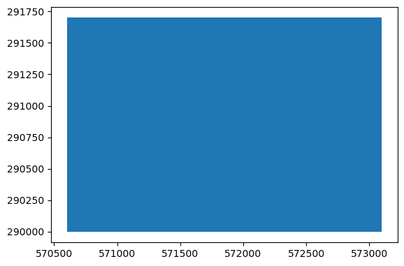
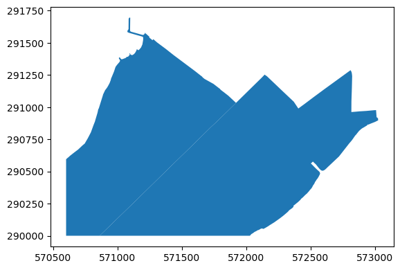
Let’s explore the various predicates with a small intersecting box
[43]:
bbox = box(570600, 290000, 573100, 291700)
bounds = gp.GeoDataFrame(geometry=[bbox],crs=parks.crs)
bounds.plot()
[43]:
<Axes: >
See documentation for full set of options for predicates. We’ll just check out a couple options: intersects, contains, within
TEST YOUR SKILLS #1
Using the bounds geodataframe you just made, write a function to visualize predicate behaviors.
your function should accept a left geodataframe, a right geodataframe, and a string for the predicate
your function should plot:
the left geodataframe in (default) blue
the result of the spatial join operation in another color
the right geodataframe in another color with outline only
then you should set the title of the plot to the string predicate value used
the geodataframes to test with are
isthmus_parksandboundsyour function should
returnthe joined geodataframea couple hints:
in the
plotmethod are a couple args calledfacecolorandedgecolorthat will help plot the rectanglethere are other predicates to try out
advanced options: if that was easy, you can try a couple other things like:
explore joins with points and lines in addition to just polygons
change around the
boundspolygon dimensionsuse
explore()to make an interactive map
[ ]:
[ ]:
[ ]:
[ ]:
[ ]:
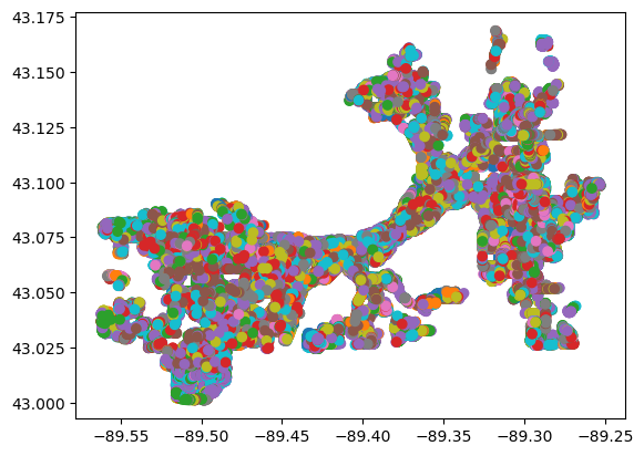
Spatial joins are particularly useful with collections of points. A common case is to add a polygon attribute to points falling within each polygon. Let’s check out a bigger point dataset with all the trees on streets in Madison
[44]:
trees = gp.read_file(datapath / 'Street_Trees.geojson')
trees.plot(column='SPECIES')
[44]:
<Axes: >
let’s put this into the same crs as neighborhoods and join the data together so we can have a neighborhood attribute on the trees geodataframe
[45]:
trees.to_crs(hoods.crs, inplace=True)
[46]:
hoods.columns
[46]:
Index(['OBJECTID', 'NA_ID', 'NEIGHB_NAME', 'STATUS', 'CLASSIFICA', 'Web',
       'ShapeSTArea', 'ShapeSTLength', 'geometry'],
      dtype='str')
NOTE: if we pass only some columns of the GeoDataFrame, only those columns will be included in the result, which is cool. But - must include the active geometry column as well!
[47]:
trees_with_hoods = trees[['SPECIES','DIAMETER','geometry']].sjoin(hoods[['NEIGHB_NAME','geometry']])
trees_with_hoods
[47]:
| SPECIES | DIAMETER | geometry | index_right | NEIGHB_NAME | |
|---|---|---|---|---|---|
| 0 | 554 | 22.0 | POINT (569406.122 285635.225) | 6 | Bram's Addition Neighborhood Association |
| 1 | 554 | 20.0 | POINT (569391.615 285635.545) | 6 | Bram's Addition Neighborhood Association |
| 2 | 320 | 14.0 | POINT (569383.333 285772.643) | 6 | Bram's Addition Neighborhood Association |
| 3 | 320 | 20.0 | POINT (569407.725 285782.686) | 6 | Bram's Addition Neighborhood Association |
| 4 | 320 | 20.0 | POINT (569431.459 285792.707) | 6 | Bram's Addition Neighborhood Association |
| ... | ... | ... | ... | ... | ... |
| 112506 | 462 | 2.0 | POINT (560220.817 289224.439) | 79 | Wexford Village Condominium Owners Assoc |
| 112507 | 804 | 2.0 | POINT (560124.192 289029.458) | 73 | Walnut Grove Homeowners Association |
| 112508 | 734 | 2.0 | POINT (559632.848 288907.214) | 58 | Sauk Creek Neighborhood Association |
| 112509 | 804 | 2.0 | POINT (559630.291 288945.507) | 58 | Sauk Creek Neighborhood Association |
| 112510 | 734 | 2.0 | POINT (559988.837 288833.319) | 73 | Walnut Grove Homeowners Association |
108937 rows × 5 columns
now we can do a groupby, for example, to find things like the average or max diameter of trees in each neighborhood
[48]:
trees_with_hoods.groupby('NEIGHB_NAME')['DIAMETER'].max().plot(kind='bar')
[48]:
<Axes: xlabel='NEIGHB_NAME'>
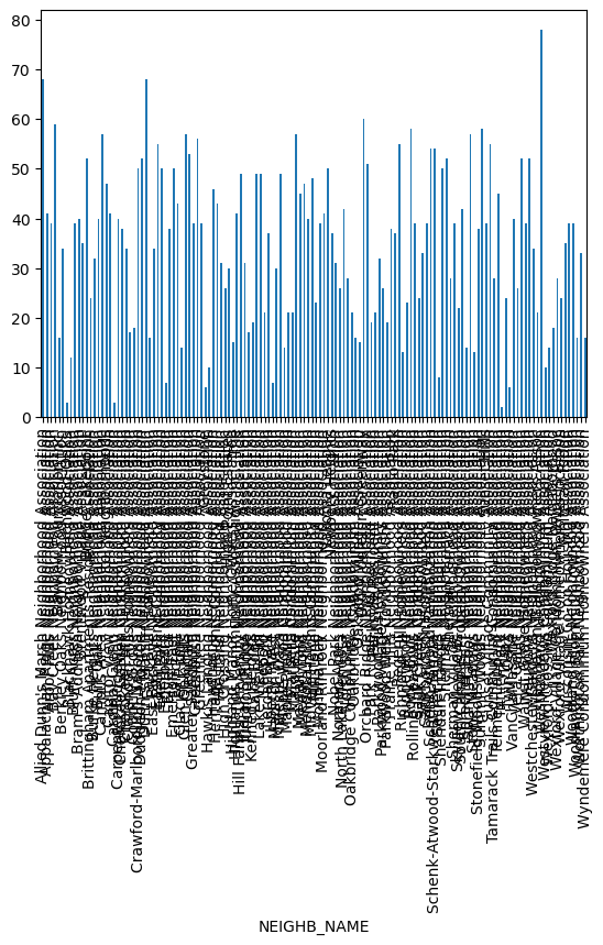
We could rearrange that bar chart in various ways, but we can also flip this back to the original neighborhoods GeoDataFrame to make a more useful spatial plot. Note that we used the spatial join to join together the attribute “Neighborhood Name” with each tree point. But now, we can aggregate those results and assign them based on an attribute rather than geospatially just like regular Pandas DataFrames
[49]:
hood_trees = hoods.copy()
tree_summary = trees_with_hoods.groupby('NEIGHB_NAME')['DIAMETER'].max()
hood_trees.merge(tree_summary,
                left_on = 'NEIGHB_NAME', right_on='NEIGHB_NAME').explore(column="DIAMETER")
[49]:
Overlays
As we’ve seen, spatial joins are powerful, but they really only gather data from multiple collections. What if we want to actually calculate the amount of overlap among shapes? Or create new shapes based on intersection or not intersection of shapes?
overlay does these things.
main options are intersection, difference, union, and symmetric_difference
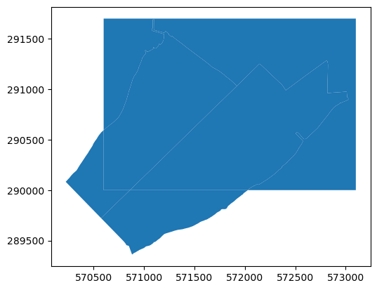
[50]:
inters = bounds.overlay(isthmus, how='intersection')
inters.plot()
[50]:
<Axes: >
[51]:
inters = bounds.overlay(isthmus, how='intersection')
inters.plot()
[51]:
<Axes: >

[52]:
inters
[52]:
| OBJECTID | NA_ID | NEIGHB_NAME | STATUS | CLASSIFICA | Web | ShapeSTArea | ShapeSTLength | geometry | |
|---|---|---|---|---|---|---|---|---|---|
| 0 | 9887 | 49 | Marquette Neighborhood Association | Active | Neighborhood Association | http://www.cityofmadison.com/neighborhoods/pro... | 1.973684e+07 | 23274.760528 | POLYGON ((570860.48 290000, 570864.33 290003.7... |
| 1 | 9915 | 92 | Tenney-Lapham Neighborhood Association | Active | Neighborhood Association | http://www.cityofmadison.com/neighborhoods/pro... | 1.333260e+07 | 18614.467212 | POLYGON ((570600 290000, 570600 290594.312, 57... |
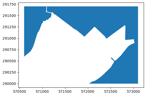
[53]:
differ = bounds.overlay(isthmus, how='difference')
differ.plot()
[53]:
<Axes: >
[54]:
differ
[54]:
| geometry | |
|---|---|
| 0 | POLYGON ((570600 291700, 573100 291700, 573100... |
[55]:
unite = bounds.overlay(isthmus, how='union')
unite.plot()
[55]:
<Axes: >
[56]:
unite
[56]:
| OBJECTID | NA_ID | NEIGHB_NAME | STATUS | CLASSIFICA | Web | ShapeSTArea | ShapeSTLength | geometry | |
|---|---|---|---|---|---|---|---|---|---|
| 0 | 9887.0 | 49.0 | Marquette Neighborhood Association | Active | Neighborhood Association | http://www.cityofmadison.com/neighborhoods/pro... | 1.973684e+07 | 23274.760528 | POLYGON ((570860.48 290000, 570864.33 290003.7... |
| 1 | 9915.0 | 92.0 | Tenney-Lapham Neighborhood Association | Active | Neighborhood Association | http://www.cityofmadison.com/neighborhoods/pro... | 1.333260e+07 | 18614.467212 | POLYGON ((570600 290000, 570600 290594.312, 57... |
| 2 | NaN | NaN | NaN | NaN | NaN | NaN | NaN | NaN | POLYGON ((570600 291700, 573100 291700, 573100... |
| 3 | 9887.0 | 49.0 | Marquette Neighborhood Association | Active | Neighborhood Association | http://www.cityofmadison.com/neighborhoods/pro... | 1.973684e+07 | 23274.760528 | POLYGON ((572028.3 289999.01, 572016.817 28999... |
| 4 | 9915.0 | 92.0 | Tenney-Lapham Neighborhood Association | Active | Neighborhood Association | http://www.cityofmadison.com/neighborhoods/pro... | 1.333260e+07 | 18614.467212 | POLYGON ((570717.845 289861.621, 570574.454 28... |
[57]:
symdiff = bounds.overlay(isthmus, how='symmetric_difference')
symdiff.plot()
[57]:
<Axes: >
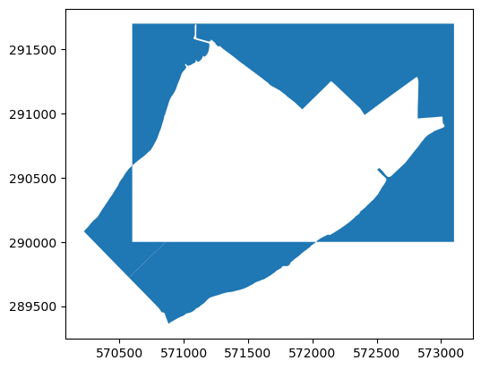
[58]:
symdiff
[58]:
| OBJECTID | NA_ID | NEIGHB_NAME | STATUS | CLASSIFICA | Web | ShapeSTArea | ShapeSTLength | geometry | |
|---|---|---|---|---|---|---|---|---|---|
| 0 | NaN | NaN | NaN | NaN | NaN | NaN | NaN | NaN | POLYGON ((570600 291700, 573100 291700, 573100... |
| 1 | 9887.0 | 49.0 | Marquette Neighborhood Association | Active | Neighborhood Association | http://www.cityofmadison.com/neighborhoods/pro... | 1.973684e+07 | 23274.760528 | POLYGON ((572028.3 289999.01, 572016.817 28999... |
| 2 | 9915.0 | 92.0 | Tenney-Lapham Neighborhood Association | Active | Neighborhood Association | http://www.cityofmadison.com/neighborhoods/pro... | 1.333260e+07 | 18614.467212 | POLYGON ((570717.845 289861.621, 570574.454 28... |
On your own…
what if you switch left and right dataframes?
how can you evaluate the areas of overlap for the intersection case?
We have an Excel file that contains a crosswalk between SPECIES number as provided and species name. Can we bring that into our dataset and evaluate some conclusions about tree species by neighborhood?
start with the
trees_with_hoodsGeoDataFrameload up and join the data from datapath / ‘Madison_Tree_Species_Lookup.xlsx’
hint: check the dtypes before merging - if you are going to join on a column, the column must be the same dtype in both dataframes
Make a multipage PDF with a page for each neighborhood showing a bar chart of the top ten tree species (by name) in each neighborhood
Make a map (use explore, or save to SHP or geojson) showing the neighborhoods with a color-coded field showing the most common tree species for each neighborhood
You will need a few pandas operations that we have only touched on a bit:
groupby, count, merge, read_excel, sort_values, iloc
[ ]: