09: Geopandas exercise solutions

import os
import numpy as np
import pandas as pd
import geopandas as gp
from shapely.geometry import Point, Polygon
from pathlib import Path
import matplotlib.pyplot as plt
from matplotlib.backends.backend_pdf import PdfPages

datapath = Path('../data/geopandas/')

TEST YOUR SKILLS #0

• make a new geodataframe of the parks

• add a columns with centroids for each park

• plot an interactive window with the park centroids and the neighborhoods

• hints:

  • remember the shapely methods are available for each geometry object (e.g. centroid())

  • you can loop over the column in a couple different ways

  • you can define which columns contains the geometry of a geodataframe

  • you will likely have to define the CRS

parks = gp.read_file(datapath / 'Madison_Parks.geojson')
hoods = gp.read_file(datapath / 'Neighborhood_Associations.geojson')

# loopy solution
parks_cent = parks.copy()
centroids = []
for i in parks_cent.geometry.values:
    centroids.append(i.centroid)
parks_cent['centroid'] = centroids

# do it all at once with a list comprehension
parks_cent['centroid'] = [i.centroid for i in parks_cent.geometry]

# set the geometry and CRS
parks_cent.set_geometry('centroid', inplace=True)
parks_cent.set_crs(parks.crs, inplace=True);

m_hoods = hoods.explore()
parks_cent.explore(m=m_hoods)

Make this Notebook Trusted to load map: File -> Trust Notebook

TEST YOUR SKILLS #1

Using the bounds geodataframe you just made, write a function to visualize predicate behaviors. - your function should accept a left geodataframe, a right geodataframe, and a string for the predicate - your function should plot: - the left geodataframe in (default) blue - the result of the spatial join operation in another color - the right geodataframe in another color with outline only - then you should set the title of the plot to the string predicate value used - the geodataframes to test with are isthmus_parks and bounds - your function should return the joined geodataframe

• a couple hints:

  • in the plot method are a couple args called facecolor and edgecolor that will help plot the rectangle

  • there are other predicates to try out

• advanced options: if that was easy, you can try a couple other things like:

  • explore joins with points and lines in addition to just polygons

  • change around the bounds polygon dimensions

  • use explore() to make an interactive map

first have to bring over some things from the main lesson

parks.to_crs(3071, inplace=True)
hoods.to_crs(parks.crs, inplace=True)
isthmus = hoods.loc[hoods['NEIGHB_NAME'].str.contains('Marquette') |
                   hoods['NEIGHB_NAME'].str.contains('Tenney')]
from shapely.geometry import box
bbox = box(570600, 290000, 573100, 291700)
bounds = gp.GeoDataFrame(geometry=[bbox],crs=parks.crs)
isthmus_parks = gp.sjoin(left_df=parks, right_df=isthmus)
isthmus_parks.drop(columns=[ 'index_right','OBJECTID_right', 'NA_ID', 'STATUS', 'CLASSIFICA', 'Web',
       'ShapeSTArea', 'ShapeSTLength'], inplace=True)

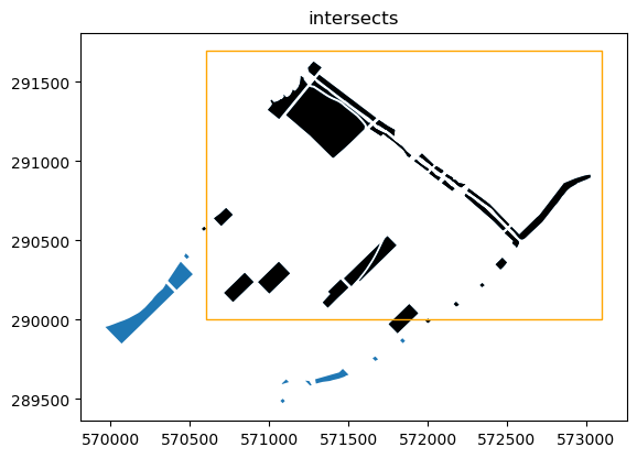
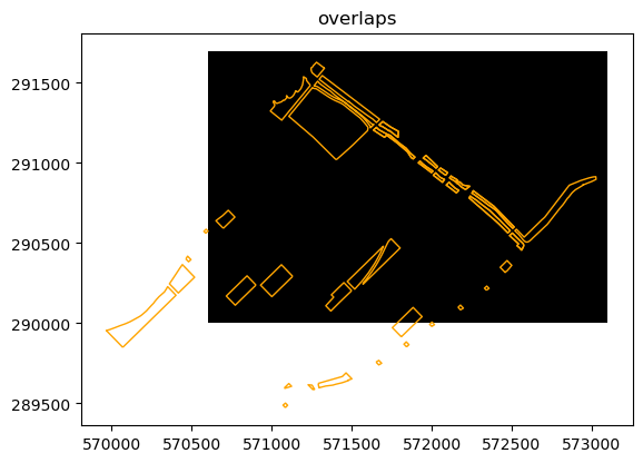
def show_predicate(ldf,rdf,predicate):
    sj = gp.sjoin(ldf, rdf, predicate=predicate)
    ax = ldf.plot()
    sj.plot(ax=ax, color='black')
    rdf.plot(facecolor='none', edgecolor='orange', ax=ax)
    ax.set_title(predicate)
    return sj

sj = show_predicate(isthmus_parks, bounds, 'intersects')
sj.head()

	OBJECTID_left	Park_ID	Type	Acreage	Park_Name	ShortName	Subtype	SHAPESTArea	SHAPESTLength	geometry	NEIGHB_NAME	index_right
6	6422	1360	NEIGHBORHOOD	6.08	Yahara Place Park	Yahara Place	None	264814.254303	4619.706039	POLYGON ((572969.327 290871.975, 572979.154 29...	Marquette Neighborhood Association	0
12	6428	3540	TRAFFICWAY	0.10	Few Street (South) Street End	Few St	None	4522.502594	270.158029	POLYGON ((572000.229 289978.256, 572017.381 28...	Marquette Neighborhood Association	0
19	6435	3480	TRAFFICWAY	0.12	Baldwin Street End	Baldwin St	None	5319.010742	294.682954	POLYGON ((572164.248 290098.321, 572179.960 29...	Marquette Neighborhood Association	0
49	6465	1240	MINI	0.66	Morrison Park	Morrison	None	28667.633148	680.142299	POLYGON ((572460.118 290317.086, 572465.604 29...	Marquette Neighborhood Association	0
56	6472	1100	OPEN SPACE	7.66	Yahara River Parkway	Yahara River	None	333593.558197	13219.124814	MULTIPOLYGON (((572463.071 290603.880, 572425....	Marquette Neighborhood Association	0

sj = show_predicate(bounds, isthmus_parks, 'overlaps')
sj.head()

	geometry	index_right	OBJECTID_left	Park_ID	Type	Acreage	Park_Name	ShortName	Subtype	SHAPESTArea	SHAPESTLength	NEIGHB_NAME
0	POLYGON ((573100.000 290000.000, 573100.000 29...	35	6451	3590	TRAFFICWAY	0.08	Paterson Street (North) Street End	Paterson St	None	3549.678101	239.046579	Tenney-Lapham Neighborhood Association
0	POLYGON ((573100.000 290000.000, 573100.000 29...	12	6428	3540	TRAFFICWAY	0.10	Few Street (South) Street End	Few St	None	4522.502594	270.158029	Marquette Neighborhood Association
0	POLYGON ((573100.000 290000.000, 573100.000 29...	92	6509	1000	MINI	3.58	Orton Park	Orton	None	156086.664276	1712.836076	Marquette Neighborhood Association

TEST YOUR SKILLS OPTIONAL

We have an Excel file that contains a crosswalk between SPECIES number as provided and species name. Can we bring that into our dataset and evaluate some conclusions about tree species by neighborhood? - start with the trees_with_hoods GeoDataFrame - load up and join the data from datapath / ‘Madison_Tree_Species_Lookup.xlsx’ - hint: check the dtypes before merging - if you are going to join on a column, the column must be the same dtype in both dataframes - Make a multipage PDF with a page for each neighborhood showing a bar chart of the top ten tree species (by name) in each neighborhood - Make a map (use explore, or save to SHP or geojson) showing the neighborhoods with a color-coded field showing the most common tree species for each neighborhood

You will need a few pandas operations that we have only touched on a bit:

groupby, count, merge, read_excel, sort_values, iloc

# read back in the trees and hoods data
trees = gp.read_file(datapath / 'Street_Trees.geojson', index_col=0)
trees.to_crs(hoods.crs, inplace=True)
trees_with_hoods = trees[['SPECIES','DIAMETER','geometry']].sjoin(hoods[['NEIGHB_NAME','geometry']])
trees_with_hoods.head()

	SPECIES	DIAMETER	geometry	index_right	NEIGHB_NAME
0	554	22.0	POINT (569406.122 285635.225)	6	Bram's Addition Neighborhood Association
1	554	20.0	POINT (569391.615 285635.545)	6	Bram's Addition Neighborhood Association
2	320	14.0	POINT (569383.333 285772.643)	6	Bram's Addition Neighborhood Association
3	320	20.0	POINT (569407.725 285782.686)	6	Bram's Addition Neighborhood Association
4	320	20.0	POINT (569431.459 285792.707)	6	Bram's Addition Neighborhood Association

# now read the excel file with tree species lookup - might need to fiddle with skiprows parameter
tree_species = pd.read_excel(datapath / 'Madison_Tree_Species_Lookup.xlsx',
                             skiprows = 6)
tree_species

	Code	Description
0	768	Cherry 'Pink Flair'
1	769	Amur Chokecherry
2	762	Black Cherry
3	666	Crabapple 'Adirondack'
4	665	Crabapple 'Sugar Tyme'
...	...	...
248	800	Oak Spp.
249	681	White Mulberry
250	680	Mulberry Spp.
251	805	Buckthorn Spp.
252	804	Swamp White Oak

253 rows × 2 columns

# check out the data types
tree_species.dtypes

Code            int64
Description    object
dtype: object

trees_with_hoods.dtypes

SPECIES          object
DIAMETER        float64
geometry       geometry
index_right       int64
NEIGHB_NAME      object
dtype: object

# d'oh! Code in tree_species and SPECIES in trees_with_hoods are different types.
# To make them consistent, let's convert SPECIES in trees_with_hoods to int
trees_with_hoods.SPECIES = [int(i) for i in trees_with_hoods.SPECIES]

trees_with_hoods.dtypes

SPECIES           int64
DIAMETER        float64
geometry       geometry
index_right       int64
NEIGHB_NAME      object
dtype: object

# now we can merge - check out the left_on, right_on args
trees_final = trees_with_hoods.merge(tree_species, left_on='SPECIES', right_on='Code')
trees_final

	SPECIES	DIAMETER	geometry	index_right	NEIGHB_NAME	Code	Description
0	554	22.0	POINT (569406.122 285635.225)	6	Bram's Addition Neighborhood Association	554	Honeylocust Var.
1	554	20.0	POINT (569391.615 285635.545)	6	Bram's Addition Neighborhood Association	554	Honeylocust Var.
2	554	8.0	POINT (569453.239 285930.349)	6	Bram's Addition Neighborhood Association	554	Honeylocust Var.
3	554	17.0	POINT (569463.866 285930.348)	6	Bram's Addition Neighborhood Association	554	Honeylocust Var.
4	554	20.0	POINT (569478.882 285930.117)	6	Bram's Addition Neighborhood Association	554	Honeylocust Var.
...	...	...	...	...	...	...	...
109750	976	19.0	POINT (568756.395 285356.696)	11	Burr Oaks Neighborhood Association	976	Elm 'Regal'
109751	976	15.0	POINT (568814.361 285356.511)	11	Burr Oaks Neighborhood Association	976	Elm 'Regal'
109752	976	10.0	POINT (568827.546 285356.119)	11	Burr Oaks Neighborhood Association	976	Elm 'Regal'
109753	80	4.0	POINT (566329.451 283988.236)	2	Arbor Hills Neighborhood Association	80	Dawn Redwood
109754	80	4.0	POINT (566329.451 283988.236)	2	Arbor Hills Neighborhood Association	80	Dawn Redwood

109755 rows × 7 columns

# now the multipage plots
with PdfPages(datapath / 'TreePlots.pdf') as outpdf:
    # first groupby neighborhoods
    for cn, cg in trees_final.groupby('NEIGHB_NAME'):
        #then, for each neighborhood, group by "Description" to get counts by name
        counts = cg.groupby('Description')['SPECIES'].count()
        # sort them in reverse value
        counts.sort_values(ascending=False, inplace=True)
        #make a bar chart of the top ten counts
        counts[:10].plot.bar()
        # set up a title
        plt.title(f'top 10 trees in {cn}')
        # when the x-axis labels are long they can get cut off. tight_layout can help
        plt.tight_layout()
        outpdf.savefig()
        plt.close('all')

# we can do this in an extra-pythonic way as well, chaining operations together
# advantage is it's faster to run but can be harder to initially understand and debug
with PdfPages(datapath / 'TreePlots.pdf') as outpdf:
    # first groupby neighborhoods
    for cn, cg in trees_final.groupby('NEIGHB_NAME'):
        cg.groupby('Description')['SPECIES'].count().sort_values(ascending=False)[:10].plot.bar()
        # set up a title
        plt.title(f'top 10 trees in {cn}')
        # when the x-axis labels are long they can get cut off. tight_layout can help
        plt.tight_layout()
        outpdf.savefig()
        plt.close('all')

Now let’s find the most common tree species in each neighborhood and make a map. There are some “sophisticated” ways using lots of pandas intrinsic functionality that can work, but we can also do it in a few (hopefully) logical explicit steps.

# we can make a couple empty lists and just append the neighborhood name and the index of the
# maximum occurring tree species in each in a loop. Still some "cleverness"
hood = []
max_tree = []
for cn, cg in trees_final.groupby('NEIGHB_NAME'):
    hood.append(cn)
    max_tree.append(cg.groupby('Description').count().sort_values(by='SPECIES', ascending=False).iloc[0].name)

# make a dataframe with these values
mts = pd.DataFrame(index=hood, data={'max_tree':max_tree})

#now join this back into the GeoDataFrame of hoods
hoods.merge(mts, left_on='NEIGHB_NAME', right_index=True)[['NEIGHB_NAME','max_tree', 'geometry']].explore(column='max_tree')

Make this Notebook Trusted to load map: File -> Trust Notebook