05: NumPy exercise solutions
[1]:
import os
from pathlib import Path
import matplotlib.pyplot as plt
import numpy as np
#this line sets up the directory paths that we will be using
datapath = Path('../data/numpy/')
print('Data will be loaded from the following directory: ', datapath)
Data will be loaded from the following directory: ../data/numpy
TEST YOUR SKILLS #0
Write the Mt. St. Helens array (before) to a new file called
mynewarray.datin the same folder asmt_st_helens_before.dat. Explore different formats (see the note under documentation for more) and see if you can read it back in again. What are the file size ramifications of format choices?Take a look at
bottom_commented.datin a text editor. What about this file? Can you read this file usingloadtxtwithout having to manually change the file? Hint: look at theloadtxtarguments.
part 0.0
[2]:
before = np.loadtxt(datapath / 'mt_st_helens_before.dat', dtype=np.float32)
[3]:
np.savetxt(datapath / 'mynewarray.dat', before, fmt='%4.3f')
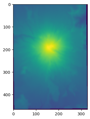
[4]:
b4 = np.loadtxt(datapath / 'mynewarray.dat')
plt.imshow(b4)
[4]:
<matplotlib.image.AxesImage at 0x7ff2242f3a10>
[5]:
# how about the built-in binary formats?
np.save(datapath / 'tmpfile', before)
[6]:
b4_2 = np.load(datapath / 'tmpfile.npy')
[7]:
plt.imshow(b4_2)
[7]:
<matplotlib.image.AxesImage at 0x7ff224367b10>

part 0.1
[8]:
filename = datapath / 'bottom_commented.dat'
[9]:
bots = np.loadtxt(filename, comments = '!')
plt.imshow(bots)
[9]:
<matplotlib.image.AxesImage at 0x7ff1f4d99810>
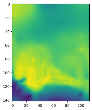
what happens if you don’t include the comment argument?
TEST YOUR SKILLS #1
Let’s calculate the amount of material lost from Mt. St. Helens in the 1980 eruption. We have the before and after elevation arrays in the data folder noted in the next cell. We will need to load them up.
The before and after files are the same dimensions, but they have some zeros around the edges indicating “nodata” values.
Check to see - are the zeros in the same place in both arrays? (
np.whereand friends can help with that).If there are no-data zeros in one array at a different location than the other array, what happens if you look at the difference?
assume each pixel is 25 x 25 feet and the elevation arrays are provided in meters to calculate a volumetric difference between before and after arrays.
[10]:
before_file = datapath / 'mt_st_helens_before.dat'
after_file = datapath / 'mt_st_helens_after.dat'
[11]:
before = np.loadtxt(before_file)
after = np.loadtxt(after_file)
# convert from meters to feet (!)
before *= 3.28084
after *= 3.28084
[12]:
np.sum((before-after) * 25 * 25)
[12]:
np.float64(3887120777.2749996)
are there the same number of 0 values in each array?
[13]:
# compare np.where results
# use np.where
print('using np.where')
print(len(np.where(before==0)[0]) , len(np.where(after==0)[0]))
using np.where
3557 3497
d’oh! not the same …. what to do?
[14]:
# we need to find the values where EITHER after is 0 or before is 0 and deal with them somehow
zero_args = np.where((before==0) | (after==0))
zero_args
[14]:
(array([  0,   0,   0, ..., 465, 465, 465], shape=(3824,)),
 array([  0,   1,   2, ..., 324, 325, 326], shape=(3824,)))
[15]:
# or we can find good locations (note the "and" rather than "or" here...)
good_args = np.where((before!=0) & (after!=0))
good_args
[15]:
(array([  0,   0,   0, ..., 464, 464, 464], shape=(148558,)),
 array([261, 262, 263, ...,  63,  64,  65], shape=(148558,)))
[16]:
np.prod(before.shape)
[16]:
np.int64(152382)
[17]:
len(zero_args[0])+len(good_args[0])
[17]:
152382
[18]:
# we could use the good_args mask to only compare the valid data and leave the nodata (and their differences) as 0
np.sum((before[good_args]-after[good_args]) * 25 * 25)
[18]:
np.float64(3919412444.9750004)
[19]:
# Or how about we set all the 0s in either array to 0, or to np.nan? What will happen when we subtract?
[20]:
before[zero_args] = 0
after[zero_args] = 0
[21]:
np.sum((before-after) * 25 * 25)
[21]:
np.float64(3919412444.9750004)
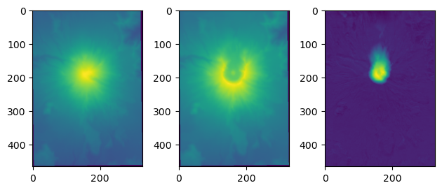
[22]:
# this second option makes it easier to make a plot of the results
fig, ax = plt.subplots(1,3)
ax[0].imshow(before)
ax[1].imshow(after)
ax[2].imshow(before-after)
plt.tight_layout()
[23]:
# or we can take advantage of the behavior of nan (not a number)
before = np.loadtxt(before_file)
after = np.loadtxt(after_file)
# convert from meters to feet (!)
before *= 3.28084
after *= 3.28084
[24]:
# first note that the result of doing any math with nan returns nan
1-np.nan
[24]:
nan
[25]:
# so, we can just convert all the 0 values in both arrays to np.nan and subtract
before[before==0] = np.nan
after[after==0] = np.nan
diff = before-after
np.nansum(diff) * 25*25
[25]:
np.float64(3919412444.975)
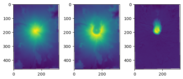
[26]:
# this second option makes it easier to make a plot of the results
fig, ax = plt.subplots(1,3)
ax[0].imshow(before)
ax[1].imshow(after)
ax[2].imshow(before-after)
plt.tight_layout()
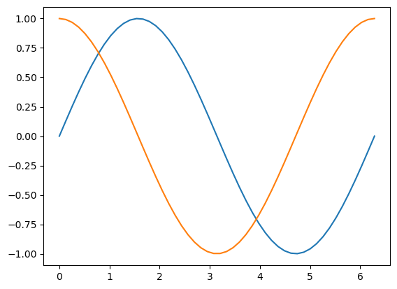
TEST YOUR SKILLS #2
In an earlier exercise, you made x and y using the following lines of code. Now use vstack to add another row to y that has the cosine of x. Then plot them both on the same figure.
hint
plt.plot(x,y)makes plots of arrays x and y
[27]:
x = np.linspace(0, 2*np.pi)
y = np.sin(x)
[28]:
y2 = np.cos(x)
[29]:
# using vstack
yy2 = np.vstack((y,y2))
yy2
[29]:
array([[ 0.00000000e+00,  1.27877162e-01,  2.53654584e-01,
         3.75267005e-01,  4.90717552e-01,  5.98110530e-01,
         6.95682551e-01,  7.81831482e-01,  8.55142763e-01,
         9.14412623e-01,  9.58667853e-01,  9.87181783e-01,
         9.99486216e-01,  9.95379113e-01,  9.74927912e-01,
         9.38468422e-01,  8.86599306e-01,  8.20172255e-01,
         7.40277997e-01,  6.48228395e-01,  5.45534901e-01,
         4.33883739e-01,  3.15108218e-01,  1.91158629e-01,
         6.40702200e-02, -6.40702200e-02, -1.91158629e-01,
        -3.15108218e-01, -4.33883739e-01, -5.45534901e-01,
        -6.48228395e-01, -7.40277997e-01, -8.20172255e-01,
        -8.86599306e-01, -9.38468422e-01, -9.74927912e-01,
        -9.95379113e-01, -9.99486216e-01, -9.87181783e-01,
        -9.58667853e-01, -9.14412623e-01, -8.55142763e-01,
        -7.81831482e-01, -6.95682551e-01, -5.98110530e-01,
        -4.90717552e-01, -3.75267005e-01, -2.53654584e-01,
        -1.27877162e-01, -2.44929360e-16],
       [ 1.00000000e+00,  9.91790014e-01,  9.67294863e-01,
         9.26916757e-01,  8.71318704e-01,  8.01413622e-01,
         7.18349350e-01,  6.23489802e-01,  5.18392568e-01,
         4.04783343e-01,  2.84527587e-01,  1.59599895e-01,
         3.20515776e-02, -9.60230259e-02, -2.22520934e-01,
        -3.45365054e-01, -4.62538290e-01, -5.72116660e-01,
        -6.72300890e-01, -7.61445958e-01, -8.38088105e-01,
        -9.00968868e-01, -9.49055747e-01, -9.81559157e-01,
        -9.97945393e-01, -9.97945393e-01, -9.81559157e-01,
        -9.49055747e-01, -9.00968868e-01, -8.38088105e-01,
        -7.61445958e-01, -6.72300890e-01, -5.72116660e-01,
        -4.62538290e-01, -3.45365054e-01, -2.22520934e-01,
        -9.60230259e-02,  3.20515776e-02,  1.59599895e-01,
         2.84527587e-01,  4.04783343e-01,  5.18392568e-01,
         6.23489802e-01,  7.18349350e-01,  8.01413622e-01,
         8.71318704e-01,  9.26916757e-01,  9.67294863e-01,
         9.91790014e-01,  1.00000000e+00]])
[30]:
plt.plot(x,yy2[0])
plt.plot(x,yy2[1])
[30]:
[<matplotlib.lines.Line2D at 0x7ff1f1b1d2b0>]
[31]:
# using hstack
yy2 = np.hstack((y,y2))
yy2
[31]:
array([ 0.00000000e+00,  1.27877162e-01,  2.53654584e-01,  3.75267005e-01,
        4.90717552e-01,  5.98110530e-01,  6.95682551e-01,  7.81831482e-01,
        8.55142763e-01,  9.14412623e-01,  9.58667853e-01,  9.87181783e-01,
        9.99486216e-01,  9.95379113e-01,  9.74927912e-01,  9.38468422e-01,
        8.86599306e-01,  8.20172255e-01,  7.40277997e-01,  6.48228395e-01,
        5.45534901e-01,  4.33883739e-01,  3.15108218e-01,  1.91158629e-01,
        6.40702200e-02, -6.40702200e-02, -1.91158629e-01, -3.15108218e-01,
       -4.33883739e-01, -5.45534901e-01, -6.48228395e-01, -7.40277997e-01,
       -8.20172255e-01, -8.86599306e-01, -9.38468422e-01, -9.74927912e-01,
       -9.95379113e-01, -9.99486216e-01, -9.87181783e-01, -9.58667853e-01,
       -9.14412623e-01, -8.55142763e-01, -7.81831482e-01, -6.95682551e-01,
       -5.98110530e-01, -4.90717552e-01, -3.75267005e-01, -2.53654584e-01,
       -1.27877162e-01, -2.44929360e-16,  1.00000000e+00,  9.91790014e-01,
        9.67294863e-01,  9.26916757e-01,  8.71318704e-01,  8.01413622e-01,
        7.18349350e-01,  6.23489802e-01,  5.18392568e-01,  4.04783343e-01,
        2.84527587e-01,  1.59599895e-01,  3.20515776e-02, -9.60230259e-02,
       -2.22520934e-01, -3.45365054e-01, -4.62538290e-01, -5.72116660e-01,
       -6.72300890e-01, -7.61445958e-01, -8.38088105e-01, -9.00968868e-01,
       -9.49055747e-01, -9.81559157e-01, -9.97945393e-01, -9.97945393e-01,
       -9.81559157e-01, -9.49055747e-01, -9.00968868e-01, -8.38088105e-01,
       -7.61445958e-01, -6.72300890e-01, -5.72116660e-01, -4.62538290e-01,
       -3.45365054e-01, -2.22520934e-01, -9.60230259e-02,  3.20515776e-02,
        1.59599895e-01,  2.84527587e-01,  4.04783343e-01,  5.18392568e-01,
        6.23489802e-01,  7.18349350e-01,  8.01413622e-01,  8.71318704e-01,
        9.26916757e-01,  9.67294863e-01,  9.91790014e-01,  1.00000000e+00])
[32]:
plt.plot(x,yy2[0:len(x)])
plt.plot(x,yy2[len(x):])
[32]:
[<matplotlib.lines.Line2D at 0x7ff1f1b66cf0>]

[ ]:
[ ]: