08: Working with tabular data in Pandas

Not that type of Panda – Python’s Pandas package
Pandas is a powerful, flexible and easy to use open source data analysis and manipulation tool. Pandas is commonly used for operations that would normally be done in a spreadsheet environment and includes powerful data analysis and manipulation tools.
Let’s begin by importing the libraries and setting our data path
[1]:
from pathlib import Path
import numpy as np
import matplotlib as mpl
import matplotlib.pyplot as plt
import pandas as pd
import statsmodels.api as sm
from dataretrieval import nwis
from matplotlib.backends.backend_pdf import PdfPages
from scipy.signal import detrend

data_path = Path("..", "data", "pandas")
Get site information data for part of the Russian River near Guerneville, CA from NWIS
[2]:
bbox = (-123.10, 38.45, -122.90, 38.55)
info, metadata = nwis.get_info(bBox=[str(i) for i in bbox])
if 'geometry' in list(info):
    # dataretreival now returns as geopandas dataframe, drop "geometry" column for this example
    info.drop(columns=["geometry"], inplace=True)
/tmp/ipykernel_10575/1777507504.py:2: DeprecationWarning: `nwis.get_info` is deprecated and will be removed from `dataretrieval` on or after 2027-05-06; use `waterdata.get_monitoring_locations()` instead.
  info, metadata = nwis.get_info(bBox=[str(i) for i in bbox])
[3]:
info.to_csv(data_path / "site_info.csv", index=False)
info.head()
[3]:
| agency_cd | site_no | station_nm | site_tp_cd | lat_va | long_va | dec_lat_va | dec_long_va | coord_meth_cd | coord_acy_cd | ... | local_time_fg | reliability_cd | gw_file_cd | nat_aqfr_cd | aqfr_cd | aqfr_type_cd | well_depth_va | hole_depth_va | depth_src_cd | project_no | |
|---|---|---|---|---|---|---|---|---|---|---|---|---|---|---|---|---|---|---|---|---|---|
| 0 | USGS | 11467000 | RUSSIAN R A HACIENDA BRIDGE NR GUERNEVILLE CA | ST | 383031.0 | 1225536.0 | 38.508482 | -122.927734 | M | F | ... | Y | NaN | NNNNNNNN | NaN | NaN | NaN | NaN | NaN | NaN | NaN |
| 1 | USGS | 11467002 | RUSSIAN R A JOHNSONS BEACH A GUERNEVILLE CA | ST | 382958.0 | 1225950.0 | 38.499358 | -122.998333 | M | F | ... | Y | NaN | NNNNNNNN | NaN | NaN | NaN | NaN | NaN | NaN | 967760420 |
| 2 | USGS | 11467006 | RUSSIAN R A VACATION BEACH CA | ST | 382903.0 | 1230041.0 | 38.484080 | -123.012500 | M | F | ... | Y | NaN | NNNNNNNN | NaN | NaN | NaN | NaN | NaN | NaN | 967760420 |
| 3 | USGS | 11467050 | BIG AUSTIN C A CAZADERO CA | ST | 383215.0 | 1230518.0 | 38.537413 | -123.089447 | M | F | ... | Y | NaN | NNNNNNNN | NaN | NaN | NaN | NaN | NaN | NaN | NaN |
| 4 | USGS | 11467200 | AUSTIN C NR CAZADERO CA | ST | 383024.0 | 1230407.0 | 38.506536 | -123.069683 | M | S | ... | Y | NaN | NNNNNNNN | NaN | NaN | NaN | NaN | NaN | NaN | 967700102 |
5 rows × 42 columns
Wow that’s a lot of gages in this location, let’s info on all of them and then use this data to learn about pandas
The data returned to us from our NWIS query info was returned to us as pandas DataFrame. We’ll be working with this to start learning about the basics of pandas.
Viewing data in pandas
Pandas has built in methods to inspect DataFrame objects. We’ll look at a few handy methods:
.head(): inspect the first few rows of data.tail(): inspect the last few rows of data.index(): show the row indexes.columns(): show the column names.describe(): statistically describe the data
[4]:
info.head()
[4]:
| agency_cd | site_no | station_nm | site_tp_cd | lat_va | long_va | dec_lat_va | dec_long_va | coord_meth_cd | coord_acy_cd | ... | local_time_fg | reliability_cd | gw_file_cd | nat_aqfr_cd | aqfr_cd | aqfr_type_cd | well_depth_va | hole_depth_va | depth_src_cd | project_no | |
|---|---|---|---|---|---|---|---|---|---|---|---|---|---|---|---|---|---|---|---|---|---|
| 0 | USGS | 11467000 | RUSSIAN R A HACIENDA BRIDGE NR GUERNEVILLE CA | ST | 383031.0 | 1225536.0 | 38.508482 | -122.927734 | M | F | ... | Y | NaN | NNNNNNNN | NaN | NaN | NaN | NaN | NaN | NaN | NaN |
| 1 | USGS | 11467002 | RUSSIAN R A JOHNSONS BEACH A GUERNEVILLE CA | ST | 382958.0 | 1225950.0 | 38.499358 | -122.998333 | M | F | ... | Y | NaN | NNNNNNNN | NaN | NaN | NaN | NaN | NaN | NaN | 967760420 |
| 2 | USGS | 11467006 | RUSSIAN R A VACATION BEACH CA | ST | 382903.0 | 1230041.0 | 38.484080 | -123.012500 | M | F | ... | Y | NaN | NNNNNNNN | NaN | NaN | NaN | NaN | NaN | NaN | 967760420 |
| 3 | USGS | 11467050 | BIG AUSTIN C A CAZADERO CA | ST | 383215.0 | 1230518.0 | 38.537413 | -123.089447 | M | F | ... | Y | NaN | NNNNNNNN | NaN | NaN | NaN | NaN | NaN | NaN | NaN |
| 4 | USGS | 11467200 | AUSTIN C NR CAZADERO CA | ST | 383024.0 | 1230407.0 | 38.506536 | -123.069683 | M | S | ... | Y | NaN | NNNNNNNN | NaN | NaN | NaN | NaN | NaN | NaN | 967700102 |
5 rows × 42 columns
[5]:
info.tail()
[5]:
| agency_cd | site_no | station_nm | site_tp_cd | lat_va | long_va | dec_lat_va | dec_long_va | coord_meth_cd | coord_acy_cd | ... | local_time_fg | reliability_cd | gw_file_cd | nat_aqfr_cd | aqfr_cd | aqfr_type_cd | well_depth_va | hole_depth_va | depth_src_cd | project_no | |
|---|---|---|---|---|---|---|---|---|---|---|---|---|---|---|---|---|---|---|---|---|---|
| 23 | USGS | 383012122574501 | RUSSIAN R A ODD FELLOWS PARK NR RIO NIDO CA | ST | 383012.0 | 1225745.0 | 38.503333 | -122.962500 | G | F | ... | Y | NaN | NaN | NaN | NaN | NaN | NaN | NaN | NaN | 967760420 |
| 24 | USGS | 383016123041101 | 008N011W27N001M | GW | 383016.3 | 1230411.0 | 38.504528 | -123.069722 | G | 5 | ... | Y | C | YY Y | NaN | NaN | NaN | 30.0 | 30.0 | D | 00BHM8187 |
| 25 | USGS | 383017122580301 | 008N010W28RU01M | GW | 383017.4 | 1225802.5 | 38.504833 | -122.967361 | G | 5 | ... | Y | C | YY | NaN | NaN | NaN | 98.0 | 107.0 | D | NaN |
| 26 | USGS | 383028122554501 | HOBSON C NR HACIENDA CA | ST | 383028.0 | 1225545.0 | 38.507778 | -122.929167 | G | U | ... | Y | NaN | NaN | NaN | NaN | NaN | NaN | NaN | NaN | 967760420 |
| 27 | USGS | 383034122590701 | 008N010W29H004M | GW | 383034.4 | 1225907.9 | 38.509556 | -122.985528 | G | 5 | ... | Y | C | YY Y | N100CACSTL | NaN | NaN | 99.0 | 110.0 | D | 9677BHM32 |
5 rows × 42 columns
[6]:
# print the index names
print(info.index)
RangeIndex(start=0, stop=28, step=1)
[7]:
# print the column names
print(info.columns)

# print the column names as a list
print(list(info))
Index(['agency_cd', 'site_no', 'station_nm', 'site_tp_cd', 'lat_va', 'long_va',
       'dec_lat_va', 'dec_long_va', 'coord_meth_cd', 'coord_acy_cd',
       'coord_datum_cd', 'dec_coord_datum_cd', 'district_cd', 'state_cd',
       'county_cd', 'country_cd', 'land_net_ds', 'map_nm', 'map_scale_fc',
       'alt_va', 'alt_meth_cd', 'alt_acy_va', 'alt_datum_cd', 'huc_cd',
       'basin_cd', 'topo_cd', 'instruments_cd', 'construction_dt',
       'inventory_dt', 'drain_area_va', 'contrib_drain_area_va', 'tz_cd',
       'local_time_fg', 'reliability_cd', 'gw_file_cd', 'nat_aqfr_cd',
       'aqfr_cd', 'aqfr_type_cd', 'well_depth_va', 'hole_depth_va',
       'depth_src_cd', 'project_no'],
      dtype='str')
['agency_cd', 'site_no', 'station_nm', 'site_tp_cd', 'lat_va', 'long_va', 'dec_lat_va', 'dec_long_va', 'coord_meth_cd', 'coord_acy_cd', 'coord_datum_cd', 'dec_coord_datum_cd', 'district_cd', 'state_cd', 'county_cd', 'country_cd', 'land_net_ds', 'map_nm', 'map_scale_fc', 'alt_va', 'alt_meth_cd', 'alt_acy_va', 'alt_datum_cd', 'huc_cd', 'basin_cd', 'topo_cd', 'instruments_cd', 'construction_dt', 'inventory_dt', 'drain_area_va', 'contrib_drain_area_va', 'tz_cd', 'local_time_fg', 'reliability_cd', 'gw_file_cd', 'nat_aqfr_cd', 'aqfr_cd', 'aqfr_type_cd', 'well_depth_va', 'hole_depth_va', 'depth_src_cd', 'project_no']
The describe() method is only useful for numerical data. This example is does not have a lot of useful data for describe(), however we’ll use it again later
[8]:
info.describe()
[8]:
| lat_va | long_va | dec_lat_va | dec_long_va | district_cd | state_cd | county_cd | map_scale_fc | alt_va | alt_acy_va | huc_cd | basin_cd | construction_dt | inventory_dt | drain_area_va | contrib_drain_area_va | aqfr_cd | aqfr_type_cd | well_depth_va | hole_depth_va | |
|---|---|---|---|---|---|---|---|---|---|---|---|---|---|---|---|---|---|---|---|---|
| count | 28.000000 | 2.800000e+01 | 28.000000 | 28.000000 | 28.0 | 28.0 | 28.0 | 25.0 | 26.000000 | 26.000000 | 2.800000e+01 | 0.0 | 6.000000e+00 | 1.100000e+01 | 6.000000 | 0.0 | 0.0 | 0.0 | 9.000000 | 6.00000 |
| mean | 382918.225000 | 1.228085e+06 | 38.488771 | -122.993363 | 6.0 | 6.0 | 97.0 | 24000.0 | 41.524615 | 10.235385 | 1.931263e+10 | NaN | 1.987590e+07 | 2.009075e+07 | 935.400000 | NaN | NaN | NaN | 63.028889 | 76.50000 |
| std | 136.242381 | 2.339461e+03 | 0.022509 | 0.059290 | 0.0 | 0.0 | 0.0 | 0.0 | 40.057582 | 9.278299 | 5.672084e+10 | NaN | 5.148255e+04 | 5.980639e+04 | 691.350481 | NaN | NaN | NaN | 34.634297 | 40.79093 |
| min | 382701.000000 | 1.225404e+06 | 38.450278 | -123.089447 | 6.0 | 6.0 | 97.0 | 24000.0 | 2.000000 | 0.100000 | 1.801011e+07 | NaN | 1.983093e+07 | 2.004091e+07 | 26.600000 | NaN | NaN | NaN | 22.000000 | 22.00000 |
| 25% | 382795.625000 | 1.225627e+06 | 38.468229 | -123.049445 | 6.0 | 6.0 | 97.0 | 24000.0 | 14.582500 | 1.600000 | 1.801011e+07 | NaN | 1.984061e+07 | 2.004091e+07 | 381.600000 | NaN | NaN | NaN | 30.000000 | 42.50000 |
| 50% | 382979.950000 | 1.230018e+06 | 38.499943 | -123.004861 | 6.0 | 6.0 | 97.0 | 24000.0 | 43.260000 | 4.300000 | 1.801011e+07 | NaN | 1.985078e+07 | 2.004092e+07 | 1345.500000 | NaN | NaN | NaN | 80.000000 | 93.50000 |
| 75% | 383013.075000 | 1.230255e+06 | 38.503632 | -122.943583 | 6.0 | 6.0 | 97.0 | 24000.0 | 48.000000 | 20.000000 | 1.801011e+07 | NaN | 1.992106e+07 | 2.014561e+07 | 1366.500000 | NaN | NaN | NaN | 98.000000 | 109.25000 |
| max | 383215.000000 | 1.230518e+06 | 38.537413 | -122.901222 | 6.0 | 6.0 | 97.0 | 24000.0 | 211.000000 | 20.000000 | 1.801011e+11 | NaN | 1.994120e+07 | 2.017050e+07 | 1461.000000 | NaN | NaN | NaN | 99.000000 | 110.00000 |
Getting data from a pandas dataframe
There are multiple methods to get data out of a pandas dataframe as either a “series”, numpy array, or a list
Let’s start by getting data as a series using a few methods
[9]:
# get a series of site numbers by key
info["site_no"]
[9]:
0            11467000
1            11467002
2            11467006
3            11467050
4            11467200
5            11467210
6     382701123025801
7     382713123030401
8     382713123030403
9     382752123003401
10    382754123030501
11    382757123003801
12    382808122565401
13    382815123024601
14    382819123010001
15    382944123002901
16    382955122594101
17    383001122540701
18    383003122540401
19    383003122540402
20    383003122540403
21    383006123000601
22    383009122543001
23    383012122574501
24    383016123041101
25    383017122580301
26    383028122554501
27    383034122590701
Name: site_no, dtype: str
[10]:
# get station names by attribute
info.station_nm
[10]:
0     RUSSIAN R A HACIENDA BRIDGE NR GUERNEVILLE CA
1       RUSSIAN R A JOHNSONS BEACH A GUERNEVILLE CA
2                     RUSSIAN R A VACATION BEACH CA
3                        BIG AUSTIN C A CAZADERO CA
4                           AUSTIN C NR CAZADERO CA
5                      RUSSIAN R A DUNCANS MILLS CA
6                   FREEZEOUT C NR DUNCANS MILLS CA
7                                   007N011W14NU01M
8                                   007N011W14NU03M
9                       DUTCH BILL C A MONTE RIO CA
10     RUSSIAN R A CASINI RANCH NR DUNCANS MILLS CA
11                         RUSSIAN R A MONTE RIO CA
12                                  007N010W10H001M
13                     AUSTIN C NR DUNCANS MILLS CA
14                                  007N010W07D001M
15                      HULBERT C NR GUERNEVILLE CA
16                    POCKET CYN C A GUERNEVILLE CA
17                                  008N009W31C002M
18                                  008N009W31C003M
19                                  008N009W31C004M
20                                  008N009W31C005M
21                          FIFE C A GUERNEVILLE CA
22             GREEN VALLEY C NR MIRABEL HEIGHTS CA
23      RUSSIAN R A ODD FELLOWS PARK NR RIO NIDO CA
24                                  008N011W27N001M
25                                  008N010W28RU01M
26                          HOBSON C NR HACIENDA CA
27                                  008N010W29H004M
Name: station_nm, dtype: str
getting data from a dataframe as a numpy array can be accomplished by using .values
[11]:
info.station_nm.values
[11]:
<ArrowStringArray>
['RUSSIAN R A HACIENDA BRIDGE NR GUERNEVILLE CA',
   'RUSSIAN R A JOHNSONS BEACH A GUERNEVILLE CA',
                 'RUSSIAN R A VACATION BEACH CA',
                    'BIG AUSTIN C A CAZADERO CA',
                       'AUSTIN C NR CAZADERO CA',
                  'RUSSIAN R A DUNCANS MILLS CA',
               'FREEZEOUT C NR DUNCANS MILLS CA',
                               '007N011W14NU01M',
                               '007N011W14NU03M',
                   'DUTCH BILL C A MONTE RIO CA',
  'RUSSIAN R A CASINI RANCH NR DUNCANS MILLS CA',
                      'RUSSIAN R A MONTE RIO CA',
                               '007N010W10H001M',
                  'AUSTIN C NR DUNCANS MILLS CA',
                               '007N010W07D001M',
                   'HULBERT C NR GUERNEVILLE CA',
                 'POCKET CYN C A GUERNEVILLE CA',
                               '008N009W31C002M',
                               '008N009W31C003M',
                               '008N009W31C004M',
                               '008N009W31C005M',
                       'FIFE C A GUERNEVILLE CA',
          'GREEN VALLEY C NR MIRABEL HEIGHTS CA',
   'RUSSIAN R A ODD FELLOWS PARK NR RIO NIDO CA',
                               '008N011W27N001M',
                               '008N010W28RU01M',
                       'HOBSON C NR HACIENDA CA',
                               '008N010W29H004M']
Length: 28, dtype: str
Selection by position
We can get data by position in the dataframe using the .iloc attribute
[12]:
info.iloc[0:2, 1:4]
[12]:
| site_no | station_nm | site_tp_cd | |
|---|---|---|---|
| 0 | 11467000 | RUSSIAN R A HACIENDA BRIDGE NR GUERNEVILLE CA | ST |
| 1 | 11467002 | RUSSIAN R A JOHNSONS BEACH A GUERNEVILLE CA | ST |
Selection by label
Pandas allows the user to get data from the dataframe by index and column labels
[13]:
info.loc[0:3, ["site_no", "station_nm", "site_tp_cd"]]
[13]:
| site_no | station_nm | site_tp_cd | |
|---|---|---|---|
| 0 | 11467000 | RUSSIAN R A HACIENDA BRIDGE NR GUERNEVILLE CA | ST |
| 1 | 11467002 | RUSSIAN R A JOHNSONS BEACH A GUERNEVILLE CA | ST |
| 2 | 11467006 | RUSSIAN R A VACATION BEACH CA | ST |
| 3 | 11467050 | BIG AUSTIN C A CAZADERO CA | ST |
Boolean indexing
pandas dataframes supports boolean indexing that allows a user to create a new dataframe with only the data that meets a boolean condition defined by the user.
Let’s get a dataframe of only groundwater sites from the info dataframe
[14]:
dfgw = info[info["site_tp_cd"] == "GW"]
dfgw
[14]:
| agency_cd | site_no | station_nm | site_tp_cd | lat_va | long_va | dec_lat_va | dec_long_va | coord_meth_cd | coord_acy_cd | ... | local_time_fg | reliability_cd | gw_file_cd | nat_aqfr_cd | aqfr_cd | aqfr_type_cd | well_depth_va | hole_depth_va | depth_src_cd | project_no | |
|---|---|---|---|---|---|---|---|---|---|---|---|---|---|---|---|---|---|---|---|---|---|
| 7 | USGS | 382713123030401 | 007N011W14NU01M | GW | 382712.5 | 1230303.5 | 38.453472 | -123.050972 | G | 5 | ... | Y | C | YY Y | NaN | NaN | NaN | 81.70 | NaN | S | GGMC200 |
| 8 | USGS | 382713123030403 | 007N011W14NU03M | GW | 382712.5 | 1230303.5 | 38.453472 | -123.050972 | G | 5 | ... | Y | C | YY Y | NaN | NaN | NaN | 32.56 | NaN | S | GGMC200 |
| 12 | USGS | 382808122565401 | 007N010W10H001M | GW | 382808.5 | 1225654.2 | 38.469028 | -122.948389 | G | 5 | ... | Y | C | YY Y | NaN | NaN | NaN | 22.00 | 22.0 | D | 00BHM8187 |
| 14 | USGS | 382819123010001 | 007N010W07D001M | GW | 382819.9 | 1230100.8 | 38.472194 | -123.016889 | G | 5 | ... | Y | C | YY | N100CACSTL | NaN | NaN | 99.00 | 110.0 | D | 9677BHM32 |
| 17 | USGS | 383001122540701 | 008N009W31C002M | GW | 383001.9 | 1225407.7 | 38.500528 | -122.902139 | G | 5 | ... | Y | C | YY | N100CACSTL | NaN | NaN | 80.00 | 80.0 | D | 9677BHM32 |
| 18 | USGS | 383003122540401 | 008N009W31C003M | GW | 383003.3 | 1225404.4 | 38.500917 | -122.901222 | G | 1 | ... | Y | C | YY Y | N100CACSTL | NaN | NaN | NaN | NaN | NaN | 967760420 |
| 19 | USGS | 383003122540402 | 008N009W31C004M | GW | 383003.3 | 1225404.4 | 38.500917 | -122.901222 | G | 1 | ... | Y | C | Y | N100CACSTL | NaN | NaN | NaN | NaN | NaN | 967760420 |
| 20 | USGS | 383003122540403 | 008N009W31C005M | GW | 383003.3 | 1225404.4 | 38.500917 | -122.901222 | G | 1 | ... | Y | C | YY Y | N100CACSTL | NaN | NaN | 25.00 | NaN | S | 967760420 |
| 24 | USGS | 383016123041101 | 008N011W27N001M | GW | 383016.3 | 1230411.0 | 38.504528 | -123.069722 | G | 5 | ... | Y | C | YY Y | NaN | NaN | NaN | 30.00 | 30.0 | D | 00BHM8187 |
| 25 | USGS | 383017122580301 | 008N010W28RU01M | GW | 383017.4 | 1225802.5 | 38.504833 | -122.967361 | G | 5 | ... | Y | C | YY | NaN | NaN | NaN | 98.00 | 107.0 | D | NaN |
| 27 | USGS | 383034122590701 | 008N010W29H004M | GW | 383034.4 | 1225907.9 | 38.509556 | -122.985528 | G | 5 | ... | Y | C | YY Y | N100CACSTL | NaN | NaN | 99.00 | 110.0 | D | 9677BHM32 |
11 rows × 42 columns
Reading and writing data to .csv files
Pandas has support to both read and write many types of files. For this example we are focusing on .csv files. For information on other file types that are supported see the ten minutes to pandas tutorial documentation
For this part we’ll write a new .csv file of the groundwater sites that we found in NWIS using to_csv().
to_csv() has a bunch of handy options for writing to file. For this example, I’m going to drop the index column while writing by passing index=False
[15]:
csv_file = data_path / "RussianRiverGWsites.csv"
dfgw.to_csv(csv_file, index=False)
Now we can load the csv file back into a pandas dataframe with the read_csv() method.
[16]:
dfgw2 = pd.read_csv(csv_file)
dfgw2
[16]:
| agency_cd | site_no | station_nm | site_tp_cd | lat_va | long_va | dec_lat_va | dec_long_va | coord_meth_cd | coord_acy_cd | ... | local_time_fg | reliability_cd | gw_file_cd | nat_aqfr_cd | aqfr_cd | aqfr_type_cd | well_depth_va | hole_depth_va | depth_src_cd | project_no | |
|---|---|---|---|---|---|---|---|---|---|---|---|---|---|---|---|---|---|---|---|---|---|
| 0 | USGS | 382713123030401 | 007N011W14NU01M | GW | 382712.5 | 1230303.5 | 38.453472 | -123.050972 | G | 5 | ... | Y | C | YY Y | NaN | NaN | NaN | 81.70 | NaN | S | GGMC200 |
| 1 | USGS | 382713123030403 | 007N011W14NU03M | GW | 382712.5 | 1230303.5 | 38.453472 | -123.050972 | G | 5 | ... | Y | C | YY Y | NaN | NaN | NaN | 32.56 | NaN | S | GGMC200 |
| 2 | USGS | 382808122565401 | 007N010W10H001M | GW | 382808.5 | 1225654.2 | 38.469028 | -122.948389 | G | 5 | ... | Y | C | YY Y | NaN | NaN | NaN | 22.00 | 22.0 | D | 00BHM8187 |
| 3 | USGS | 382819123010001 | 007N010W07D001M | GW | 382819.9 | 1230100.8 | 38.472194 | -123.016889 | G | 5 | ... | Y | C | YY | N100CACSTL | NaN | NaN | 99.00 | 110.0 | D | 9677BHM32 |
| 4 | USGS | 383001122540701 | 008N009W31C002M | GW | 383001.9 | 1225407.7 | 38.500528 | -122.902139 | G | 5 | ... | Y | C | YY | N100CACSTL | NaN | NaN | 80.00 | 80.0 | D | 9677BHM32 |
| 5 | USGS | 383003122540401 | 008N009W31C003M | GW | 383003.3 | 1225404.4 | 38.500917 | -122.901222 | G | 1 | ... | Y | C | YY Y | N100CACSTL | NaN | NaN | NaN | NaN | NaN | 967760420 |
| 6 | USGS | 383003122540402 | 008N009W31C004M | GW | 383003.3 | 1225404.4 | 38.500917 | -122.901222 | G | 1 | ... | Y | C | Y | N100CACSTL | NaN | NaN | NaN | NaN | NaN | 967760420 |
| 7 | USGS | 383003122540403 | 008N009W31C005M | GW | 383003.3 | 1225404.4 | 38.500917 | -122.901222 | G | 1 | ... | Y | C | YY Y | N100CACSTL | NaN | NaN | 25.00 | NaN | S | 967760420 |
| 8 | USGS | 383016123041101 | 008N011W27N001M | GW | 383016.3 | 1230411.0 | 38.504528 | -123.069722 | G | 5 | ... | Y | C | YY Y | NaN | NaN | NaN | 30.00 | 30.0 | D | 00BHM8187 |
| 9 | USGS | 383017122580301 | 008N010W28RU01M | GW | 383017.4 | 1225802.5 | 38.504833 | -122.967361 | G | 5 | ... | Y | C | YY | NaN | NaN | NaN | 98.00 | 107.0 | D | NaN |
| 10 | USGS | 383034122590701 | 008N010W29H004M | GW | 383034.4 | 1225907.9 | 38.509556 | -122.985528 | G | 5 | ... | Y | C | YY Y | N100CACSTL | NaN | NaN | 99.00 | 110.0 | D | 9677BHM32 |
11 rows × 42 columns
Class exercise 1
Using the methods presented in this notebook create a DataFrame of surface water sites from the info dataframe, write it to a csv file named "RussianRiverSWsites.csv", and read it back in as a new DataFrame
[17]:
csv_name = data_path / "RussianRiverSWsites.csv"
dfsw = info[info.site_tp_cd == "ST"]
dfsw.to_csv(csv_name, index=False)

dfsw = pd.read_csv(csv_name)
dfsw.head()
[17]:
| agency_cd | site_no | station_nm | site_tp_cd | lat_va | long_va | dec_lat_va | dec_long_va | coord_meth_cd | coord_acy_cd | ... | local_time_fg | reliability_cd | gw_file_cd | nat_aqfr_cd | aqfr_cd | aqfr_type_cd | well_depth_va | hole_depth_va | depth_src_cd | project_no | |
|---|---|---|---|---|---|---|---|---|---|---|---|---|---|---|---|---|---|---|---|---|---|
| 0 | USGS | 11467000 | RUSSIAN R A HACIENDA BRIDGE NR GUERNEVILLE CA | ST | 383031.0 | 1225536.0 | 38.508482 | -122.927734 | M | F | ... | Y | NaN | NNNNNNNN | NaN | NaN | NaN | NaN | NaN | NaN | NaN |
| 1 | USGS | 11467002 | RUSSIAN R A JOHNSONS BEACH A GUERNEVILLE CA | ST | 382958.0 | 1225950.0 | 38.499358 | -122.998333 | M | F | ... | Y | NaN | NNNNNNNN | NaN | NaN | NaN | NaN | NaN | NaN | 967760420.0 |
| 2 | USGS | 11467006 | RUSSIAN R A VACATION BEACH CA | ST | 382903.0 | 1230041.0 | 38.484080 | -123.012500 | M | F | ... | Y | NaN | NNNNNNNN | NaN | NaN | NaN | NaN | NaN | NaN | 967760420.0 |
| 3 | USGS | 11467050 | BIG AUSTIN C A CAZADERO CA | ST | 383215.0 | 1230518.0 | 38.537413 | -123.089447 | M | F | ... | Y | NaN | NNNNNNNN | NaN | NaN | NaN | NaN | NaN | NaN | NaN |
| 4 | USGS | 11467200 | AUSTIN C NR CAZADERO CA | ST | 383024.0 | 1230407.0 | 38.506536 | -123.069683 | M | S | ... | Y | NaN | NNNNNNNN | NaN | NaN | NaN | NaN | NaN | NaN | 967700102.0 |
5 rows × 42 columns
Get timeseries data from NWIS for surface water sites
Now to start working with stream gage data from NWIS. We’re going to send all surface water sites to NWIS and get only sites with daily discharge measurements.
(11467002)
[18]:
# filter for only SW sites
dfsw = info[info.site_tp_cd == "ST"]

# create query
sites = dfsw.site_no.to_list()
pcode = "00060"
start_date = "1939-09-22"
end_date = "2023-12-31"
df, metadata = nwis.get_dv(
    sites=sites,
    start=start_date,
    end=end_date,
    parameterCd=pcode,
    multi_index=False
)
df.head()
/tmp/ipykernel_10575/912741710.py:9: DeprecationWarning: `nwis.get_dv` is deprecated and will be removed from `dataretrieval` on or after 2027-05-06; use `waterdata.get_daily()` instead.
  df, metadata = nwis.get_dv(
[18]:
| 00060_Mean | 00060_Mean_cd | site_no | |
|---|---|---|---|
| datetime | |||
| 1939-10-01 00:00:00+00:00 | 185.0 | A, e | 11467000 |
| 1939-10-02 00:00:00+00:00 | 185.0 | A, e | 11467000 |
| 1939-10-03 00:00:00+00:00 | 185.0 | A, e | 11467000 |
| 1939-10-04 00:00:00+00:00 | 185.0 | A, e | 11467000 |
| 1939-10-05 00:00:00+00:00 | 185.0 | A, e | 11467000 |
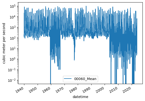
Awesome! There are two gages in this study area that have daily discharge data!
Inspect the data using .plot()
[19]:
ax = df.plot()
ax.set_ylabel(r"cubic meter per second")
ax.set_yscale("log")
Updating column names
Let’s update column names for these gages based on their locations instead of their USGS gage id. First we’ll get name information from the info class and then we’ll use the station name information to remap the column names.
the rename() method accepts a dictionary that is formatted {current_col_name: new_col_name}
[20]:
df
[20]:
| 00060_Mean | 00060_Mean_cd | site_no | |
|---|---|---|---|
| datetime | |||
| 1939-10-01 00:00:00+00:00 | 185.0 | A, e | 11467000 |
| 1939-10-02 00:00:00+00:00 | 185.0 | A, e | 11467000 |
| 1939-10-03 00:00:00+00:00 | 185.0 | A, e | 11467000 |
| 1939-10-04 00:00:00+00:00 | 185.0 | A, e | 11467000 |
| 1939-10-05 00:00:00+00:00 | 185.0 | A, e | 11467000 |
| ... | ... | ... | ... |
| 2023-12-29 00:00:00+00:00 | 1970.0 | A | 11467000 |
| 2023-12-30 00:00:00+00:00 | 6170.0 | A | 11467000 |
| 2023-12-30 00:00:00+00:00 | 1390.0 | A | 11467200 |
| 2023-12-31 00:00:00+00:00 | 5970.0 | A | 11467000 |
| 2023-12-31 00:00:00+00:00 | 619.0 | A | 11467200 |
40848 rows × 3 columns
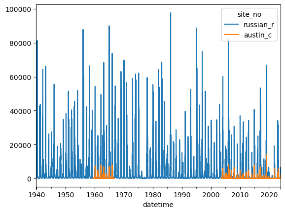
[21]:
df2 = df[['site_no', '00060_Mean']].pivot(columns=['site_no'])
df2.columns = df2.columns.get_level_values(1)

site_names = {site_no: '_'.join(name.split()[:2]).lower() for site_no, name
              in info.groupby('site_no')['station_nm'].first().loc[df2.columns].items()}
df2.rename(columns=site_names, inplace=True)
df2.plot()
[21]:
<Axes: xlabel='datetime'>
Adding a new column of data to the dataframe
Adding new columns of data is relatively simple in pandas. The call signature is similar to a dictionary where df[“key”] = “some_array_of_values”
Let’s add a year column (water year) to the dataframe by getting the year from the index and adjusting it using np.where()
[22]:
df2['year'] = np.where(df2.index.month >=10, df2.index.year, df2.index.year - 1)
Manipulating data
Columns in a pandas dataframe can be manipulated similarly to working with a dictionary of numpy arrays. The discharge data units are \(\frac{ft^3}{s}\), let’s accumulate this to daily discharge in \(\frac {ft^3}{d}\).
The conversion for this is:
$ \frac{1 ft^3}{s} \times `:nbsphinx-math:frac{60s}{min}` \times `:nbsphinx-math:frac{60min}{hour}` \times `:nbsphinx-math:frac{24hours}{day}` \rightarrow `:nbsphinx-math:frac{ft^3}{day}` $
and then convert that to acre-feet (1 acre-ft = 43559.9)
[23]:
df2
[23]:
| site_no | russian_r | austin_c | year |
|---|---|---|---|
| datetime | |||
| 1939-10-01 00:00:00+00:00 | 185.0 | NaN | 1939 |
| 1939-10-02 00:00:00+00:00 | 185.0 | NaN | 1939 |
| 1939-10-03 00:00:00+00:00 | 185.0 | NaN | 1939 |
| 1939-10-04 00:00:00+00:00 | 185.0 | NaN | 1939 |
| 1939-10-05 00:00:00+00:00 | 185.0 | NaN | 1939 |
| ... | ... | ... | ... |
| 2023-12-27 00:00:00+00:00 | 888.0 | 965.0 | 2023 |
| 2023-12-28 00:00:00+00:00 | 1640.0 | 857.0 | 2023 |
| 2023-12-29 00:00:00+00:00 | 1970.0 | 1460.0 | 2023 |
| 2023-12-30 00:00:00+00:00 | 6170.0 | 1390.0 | 2023 |
| 2023-12-31 00:00:00+00:00 | 5970.0 | 619.0 | 2023 |
30773 rows × 3 columns
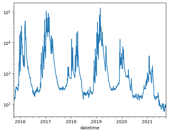
[24]:
conv = 60 * 60 * 24
df2["russian_r_cfd"] = df2.russian_r * conv
df2["russian_r_af"] = df2.russian_r_cfd / 43559.9
df2

# now let's plot up discharge from 2018 - 2020
dfplt = df2[(df2["year"] >= 2015) & (df2["year"] <= 2020)]
ax = dfplt["russian_r_af"].plot()
ax.set_yscale("log")
Class exercise 2:
Using the methods described in the notebook. Convert the discharge for "austin_c" from \(\frac{m^3}{s}\) acre-ft by adding two additional fields to df2 named "austin_c_cfs" and "austin_c_af".
After these two fields have been added to df2 use boolean indexing to create a new dataframe from 2015 through 2020. Finally plot the discharge data (in acre-ft) for “austin_cr”.
bonus exercise try to plot both "russian_r_af" and "austin_c_af" on the same plot
[25]:
conv = 60 * 60 * 24
df2["austin_c_cfd"] = df2.austin_c * conv
df2["austin_c_af"] = df2.austin_c_cfd / 43559.9
df2

# now let's plot up discharge from 2018 - 2020
dfplt = df2[(df2["year"] >= 2015) & (df2["year"] <= 2020)]
ax = dfplt["austin_c_af"].plot()
ax.set_yscale("log")
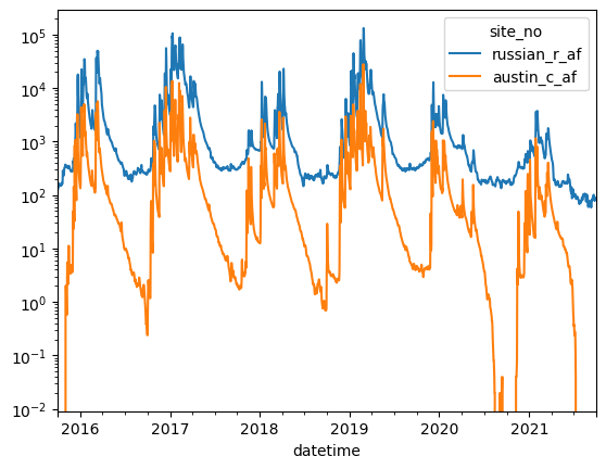
[26]:
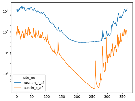
# now let's plot up discharge from 2018 - 2020
dfplt = df2[(df2["year"] >= 2015) & (df2["year"] <= 2020)]
ax = dfplt[["russian_r_af","austin_c_af"]].plot()
ax.set_yscale("log")

groupby: grouping data and performing mathematical operations on it
groupby() is a powerful method that allows for performing statistical operations over a groups of “common” data within a dataframe.
For this example we’ll use it to get mean daily flows for the watershed. Pandas will group all common days of the year with each other and then calculate the mean value of these via the function .mean(). groupby() also supports other operations such as .median(), .sum(), max(), min(), std(), and other functions.
[27]:
df2["day_of_year"] = df2.index.day_of_year

df_mean_day = df2.groupby(by=["day_of_year"], as_index=False)[["russian_r_af", "austin_c_af"]].mean()
ax = df_mean_day[["russian_r_af", "austin_c_af"]].plot()
ax.set_yscale("log")
We can see that around March flow starts decreasing heavily and doesn’t recover until sometime in october. What’s going on here? Let’s load some climate data and see what’s happening.
[28]:
cimis_file = data_path / "santa_rosa_CIMIS_83.csv"
df_cimis = pd.read_csv(cimis_file)
drop_list = ["qc"] + [f"qc.{i}" for i in range(1, 22)]
df_cimis.drop(columns=drop_list, inplace=True)
df_cimis
[28]:
| Stn Id | Stn Name | CIMIS Region | Date | Jul | ETo (in) | Precip (in) | Sol Rad (Ly/day) | Avg Vap Pres (mBars) | Max Air Temp (F) | ... | Rose NNE | Rose ENE | Rose ESE | Rose SSE | Rose SSW | Rose WSW | Rose WNW | Rose NNW | Wind Run (miles) | Avg Soil Temp (F) | |
|---|---|---|---|---|---|---|---|---|---|---|---|---|---|---|---|---|---|---|---|---|---|
| 0 | 83 | Santa Rosa | North Coast Valleys | 1/1/1990 | 1 | 0.00 | 0.30 | 42.0 | 7.7 | 48.7 | ... | 0.03 | 0.02 | 0.06 | 0.06 | 0.04 | 0.10 | 0.15 | 0.14 | 32.1 | 46.3 |
| 1 | 83 | Santa Rosa | North Coast Valleys | 1/2/1990 | 2 | 0.06 | 0.00 | 236.0 | 6.1 | 58.4 | ... | 0.06 | 0.01 | 0.04 | 0.03 | 0.03 | 0.06 | 0.45 | 1.53 | 121.0 | 44.9 |
| 2 | 83 | Santa Rosa | North Coast Valleys | 1/3/1990 | 3 | 0.04 | 0.00 | 225.0 | 5.8 | 63.0 | ... | 0.08 | 0.04 | 0.10 | 0.04 | 0.06 | 0.05 | 0.21 | 0.23 | 44.5 | 43.3 |
| 3 | 83 | Santa Rosa | North Coast Valleys | 1/4/1990 | 4 | 0.03 | 0.01 | 190.0 | 6.3 | 56.7 | ... | 0.07 | 0.07 | 0.11 | 0.07 | 0.03 | 0.03 | 0.08 | 0.09 | 30.2 | 42.8 |
| 4 | 83 | Santa Rosa | North Coast Valleys | 1/5/1990 | 5 | 0.04 | 0.00 | 192.0 | 7.2 | 59.1 | ... | 0.08 | 0.13 | 0.33 | 0.08 | 0.04 | 0.08 | 0.07 | 0.05 | 45.2 | 43.7 |
| ... | ... | ... | ... | ... | ... | ... | ... | ... | ... | ... | ... | ... | ... | ... | ... | ... | ... | ... | ... | ... | ... |
| 11948 | 83 | Santa Rosa | North Coast Valleys | 9/18/2022 | 261 | 0.03 | 0.77 | 113.0 | 16.4 | 66.8 | ... | 0.01 | 0.04 | 0.29 | 0.51 | 0.14 | 0.01 | 0.00 | 0.00 | 197.4 | 65.2 |
| 11949 | 83 | Santa Rosa | North Coast Valleys | 9/19/2022 | 262 | 0.14 | 0.02 | 424.0 | 15.6 | 73.9 | ... | 0.09 | 0.07 | 0.08 | 0.17 | 0.09 | 0.28 | 0.15 | 0.07 | 108.9 | 65.9 |
| 11950 | 83 | Santa Rosa | North Coast Valleys | 9/20/2022 | 263 | 0.10 | 0.00 | 330.0 | 13.9 | 72.6 | ... | 0.08 | 0.04 | 0.10 | 0.11 | 0.18 | 0.25 | 0.15 | 0.10 | 79.6 | 65.8 |
| 11951 | 83 | Santa Rosa | North Coast Valleys | 9/21/2022 | 264 | 0.15 | 0.07 | 458.0 | 14.8 | 75.5 | ... | 0.09 | 0.05 | 0.13 | 0.16 | 0.18 | 0.22 | 0.08 | 0.09 | 103.3 | 66.7 |
| 11952 | 83 | Santa Rosa | North Coast Valleys | 9/22/2022 | 265 | 0.17 | 0.00 | 494.0 | 13.1 | 82.9 | ... | 0.14 | 0.06 | 0.09 | 0.10 | 0.11 | 0.20 | 0.12 | 0.19 | 83.7 | 66.3 |
11953 rows × 27 columns
[29]:
df_mean_clim = df_cimis.groupby(by=["Jul"], as_index=False)[["ETo (in)", "Precip (in)"]].mean()
df_mean_clim = df_mean_clim.rename(columns={"Jul": "day_of_year"})
df_mean_clim.head()
[29]:
| day_of_year | ETo (in) | Precip (in) | |
|---|---|---|---|
| 0 | 1 | 0.031212 | 0.335455 |
| 1 | 2 | 0.031212 | 0.155152 |
| 2 | 3 | 0.030303 | 0.195484 |
| 3 | 4 | 0.030909 | 0.190303 |
| 4 | 5 | 0.034242 | 0.150000 |
Joining two DataFrames with an inner join
Inner joins can be made in pandas with the merge() method. As inner join, joins two dataframes on a common key or values, when a key or value exists in one dataframe, but not the other that row of data will be excluded from the joined dataframe.
There are a number of other ways to join dataframes in pandas. Detailed examples and discussion of the different merging methods can be found here
[30]:
df_merged = pd.merge(df_mean_day, df_mean_clim, on=["day_of_year",])
df_merged.head()
[30]:
| day_of_year | russian_r_af | austin_c_af | ETo (in) | Precip (in) | |
|---|---|---|---|---|---|
| 0 | 1 | 11169.447129 | 982.247985 | 0.031212 | 0.335455 |
| 1 | 2 | 10601.346651 | 648.518661 | 0.031212 | 0.155152 |
| 2 | 3 | 8662.758966 | 777.478369 | 0.030303 | 0.195484 |
| 3 | 4 | 9604.154280 | 1831.494379 | 0.030909 | 0.190303 |
| 4 | 5 | 11811.951556 | 1508.267191 | 0.034242 | 0.150000 |
[31]:
cols = [i for i in list(df_merged) if i != "day_of_year"]
ax = df_merged[cols].plot()
ax.set_yscale("log")
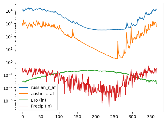
This starts to make a little more sense! We can see that this area gets most of it’s precipitation in the winter and early spring. The evapotranspiration curve shows what we’d expect: that there is more evapotranspiration in the summer than the winter.
Stepping back for a minute: exploring Merge and Concat
Merge and concat are very powerful and important methods for combining pandas DataFrames (and later geopandas GeoDataFrames). This section takes a moment, as an aside to explore some of the common funtions and options for performing merges and concatenation.
The merge method
Pandas merge method allows the user to join two dataframes based on column values. There are a few methods that can be used to control the type of merge and the result.
inner: operates as a intersection of the data and keeps rows from both dataframes if the row has a matching key in both dataframes.outer: operates as a union and joins all rows from both dataframes, fills columns with nan where data is not available for a row.left: keeps all rows from the ‘left’ dataframe and joins columns from the rightright: keeps all rows from the ‘right’ dataframe and joins columns from the left
[32]:
ex0 = {
    "name": [],
    "childhood_dream_job": []
}
ex1 = {
    "name": [],
    "age": []
}
[ ]:
[ ]:
[ ]:
The concat method
Pandas concat method allows the user to concatenate dataframes together
[33]:
gw = info[info.site_tp_cd == "GW"]
sw = info[info.site_tp_cd == "ST"]
sw = sw[list(sw)[0:8]]
sw.head()
[33]:
| agency_cd | site_no | station_nm | site_tp_cd | lat_va | long_va | dec_lat_va | dec_long_va | |
|---|---|---|---|---|---|---|---|---|
| 0 | USGS | 11467000 | RUSSIAN R A HACIENDA BRIDGE NR GUERNEVILLE CA | ST | 383031.0 | 1225536.0 | 38.508482 | -122.927734 |
| 1 | USGS | 11467002 | RUSSIAN R A JOHNSONS BEACH A GUERNEVILLE CA | ST | 382958.0 | 1225950.0 | 38.499358 | -122.998333 |
| 2 | USGS | 11467006 | RUSSIAN R A VACATION BEACH CA | ST | 382903.0 | 1230041.0 | 38.484080 | -123.012500 |
| 3 | USGS | 11467050 | BIG AUSTIN C A CAZADERO CA | ST | 383215.0 | 1230518.0 | 38.537413 | -123.089447 |
| 4 | USGS | 11467200 | AUSTIN C NR CAZADERO CA | ST | 383024.0 | 1230407.0 | 38.506536 | -123.069683 |
[34]:
newdf = pd.concat((gw, sw), ignore_index=True)
newdf
[34]:
| agency_cd | site_no | station_nm | site_tp_cd | lat_va | long_va | dec_lat_va | dec_long_va | coord_meth_cd | coord_acy_cd | ... | local_time_fg | reliability_cd | gw_file_cd | nat_aqfr_cd | aqfr_cd | aqfr_type_cd | well_depth_va | hole_depth_va | depth_src_cd | project_no | |
|---|---|---|---|---|---|---|---|---|---|---|---|---|---|---|---|---|---|---|---|---|---|
| 0 | USGS | 382713123030401 | 007N011W14NU01M | GW | 382712.5 | 1230303.5 | 38.453472 | -123.050972 | G | 5 | ... | Y | C | YY Y | NaN | NaN | NaN | 81.70 | NaN | S | GGMC200 |
| 1 | USGS | 382713123030403 | 007N011W14NU03M | GW | 382712.5 | 1230303.5 | 38.453472 | -123.050972 | G | 5 | ... | Y | C | YY Y | NaN | NaN | NaN | 32.56 | NaN | S | GGMC200 |
| 2 | USGS | 382808122565401 | 007N010W10H001M | GW | 382808.5 | 1225654.2 | 38.469028 | -122.948389 | G | 5 | ... | Y | C | YY Y | NaN | NaN | NaN | 22.00 | 22.0 | D | 00BHM8187 |
| 3 | USGS | 382819123010001 | 007N010W07D001M | GW | 382819.9 | 1230100.8 | 38.472194 | -123.016889 | G | 5 | ... | Y | C | YY | N100CACSTL | NaN | NaN | 99.00 | 110.0 | D | 9677BHM32 |
| 4 | USGS | 383001122540701 | 008N009W31C002M | GW | 383001.9 | 1225407.7 | 38.500528 | -122.902139 | G | 5 | ... | Y | C | YY | N100CACSTL | NaN | NaN | 80.00 | 80.0 | D | 9677BHM32 |
| 5 | USGS | 383003122540401 | 008N009W31C003M | GW | 383003.3 | 1225404.4 | 38.500917 | -122.901222 | G | 1 | ... | Y | C | YY Y | N100CACSTL | NaN | NaN | NaN | NaN | NaN | 967760420 |
| 6 | USGS | 383003122540402 | 008N009W31C004M | GW | 383003.3 | 1225404.4 | 38.500917 | -122.901222 | G | 1 | ... | Y | C | Y | N100CACSTL | NaN | NaN | NaN | NaN | NaN | 967760420 |
| 7 | USGS | 383003122540403 | 008N009W31C005M | GW | 383003.3 | 1225404.4 | 38.500917 | -122.901222 | G | 1 | ... | Y | C | YY Y | N100CACSTL | NaN | NaN | 25.00 | NaN | S | 967760420 |
| 8 | USGS | 383016123041101 | 008N011W27N001M | GW | 383016.3 | 1230411.0 | 38.504528 | -123.069722 | G | 5 | ... | Y | C | YY Y | NaN | NaN | NaN | 30.00 | 30.0 | D | 00BHM8187 |
| 9 | USGS | 383017122580301 | 008N010W28RU01M | GW | 383017.4 | 1225802.5 | 38.504833 | -122.967361 | G | 5 | ... | Y | C | YY | NaN | NaN | NaN | 98.00 | 107.0 | D | NaN |
| 10 | USGS | 383034122590701 | 008N010W29H004M | GW | 383034.4 | 1225907.9 | 38.509556 | -122.985528 | G | 5 | ... | Y | C | YY Y | N100CACSTL | NaN | NaN | 99.00 | 110.0 | D | 9677BHM32 |
| 11 | USGS | 11467000 | RUSSIAN R A HACIENDA BRIDGE NR GUERNEVILLE CA | ST | 383031.0 | 1225536.0 | 38.508482 | -122.927734 | NaN | NaN | ... | NaN | NaN | NaN | NaN | NaN | NaN | NaN | NaN | NaN | NaN |
| 12 | USGS | 11467002 | RUSSIAN R A JOHNSONS BEACH A GUERNEVILLE CA | ST | 382958.0 | 1225950.0 | 38.499358 | -122.998333 | NaN | NaN | ... | NaN | NaN | NaN | NaN | NaN | NaN | NaN | NaN | NaN | NaN |
| 13 | USGS | 11467006 | RUSSIAN R A VACATION BEACH CA | ST | 382903.0 | 1230041.0 | 38.484080 | -123.012500 | NaN | NaN | ... | NaN | NaN | NaN | NaN | NaN | NaN | NaN | NaN | NaN | NaN |
| 14 | USGS | 11467050 | BIG AUSTIN C A CAZADERO CA | ST | 383215.0 | 1230518.0 | 38.537413 | -123.089447 | NaN | NaN | ... | NaN | NaN | NaN | NaN | NaN | NaN | NaN | NaN | NaN | NaN |
| 15 | USGS | 11467200 | AUSTIN C NR CAZADERO CA | ST | 383024.0 | 1230407.0 | 38.506536 | -123.069683 | NaN | NaN | ... | NaN | NaN | NaN | NaN | NaN | NaN | NaN | NaN | NaN | NaN |
| 16 | USGS | 11467210 | RUSSIAN R A DUNCANS MILLS CA | ST | 382713.0 | 1230254.0 | 38.453525 | -123.049446 | NaN | NaN | ... | NaN | NaN | NaN | NaN | NaN | NaN | NaN | NaN | NaN | NaN |
| 17 | USGS | 382701123025801 | FREEZEOUT C NR DUNCANS MILLS CA | ST | 382701.0 | 1230258.0 | 38.450278 | -123.049444 | NaN | NaN | ... | NaN | NaN | NaN | NaN | NaN | NaN | NaN | NaN | NaN | NaN |
| 18 | USGS | 382752123003401 | DUTCH BILL C A MONTE RIO CA | ST | 382752.0 | 1230034.0 | 38.464444 | -123.009444 | NaN | NaN | ... | NaN | NaN | NaN | NaN | NaN | NaN | NaN | NaN | NaN | NaN |
| 19 | USGS | 382754123030501 | RUSSIAN R A CASINI RANCH NR DUNCANS MILLS CA | ST | 382754.0 | 1230305.0 | 38.465000 | -123.051389 | NaN | NaN | ... | NaN | NaN | NaN | NaN | NaN | NaN | NaN | NaN | NaN | NaN |
| 20 | USGS | 382757123003801 | RUSSIAN R A MONTE RIO CA | ST | 382757.0 | 1230038.0 | 38.465833 | -123.010556 | NaN | NaN | ... | NaN | NaN | NaN | NaN | NaN | NaN | NaN | NaN | NaN | NaN |
| 21 | USGS | 382815123024601 | AUSTIN C NR DUNCANS MILLS CA | ST | 382815.0 | 1230246.0 | 38.470833 | -123.046111 | NaN | NaN | ... | NaN | NaN | NaN | NaN | NaN | NaN | NaN | NaN | NaN | NaN |
| 22 | USGS | 382944123002901 | HULBERT C NR GUERNEVILLE CA | ST | 382944.0 | 1230029.0 | 38.495556 | -123.008056 | NaN | NaN | ... | NaN | NaN | NaN | NaN | NaN | NaN | NaN | NaN | NaN | NaN |
| 23 | USGS | 382955122594101 | POCKET CYN C A GUERNEVILLE CA | ST | 382955.0 | 1225941.0 | 38.498611 | -122.994722 | NaN | NaN | ... | NaN | NaN | NaN | NaN | NaN | NaN | NaN | NaN | NaN | NaN |
| 24 | USGS | 383006123000601 | FIFE C A GUERNEVILLE CA | ST | 383006.0 | 1230006.0 | 38.501667 | -123.001667 | NaN | NaN | ... | NaN | NaN | NaN | NaN | NaN | NaN | NaN | NaN | NaN | NaN |
| 25 | USGS | 383009122543001 | GREEN VALLEY C NR MIRABEL HEIGHTS CA | ST | 383009.0 | 1225430.0 | 38.502500 | -122.908333 | NaN | NaN | ... | NaN | NaN | NaN | NaN | NaN | NaN | NaN | NaN | NaN | NaN |
| 26 | USGS | 383012122574501 | RUSSIAN R A ODD FELLOWS PARK NR RIO NIDO CA | ST | 383012.0 | 1225745.0 | 38.503333 | -122.962500 | NaN | NaN | ... | NaN | NaN | NaN | NaN | NaN | NaN | NaN | NaN | NaN | NaN |
| 27 | USGS | 383028122554501 | HOBSON C NR HACIENDA CA | ST | 383028.0 | 1225545.0 | 38.507778 | -122.929167 | NaN | NaN | ... | NaN | NaN | NaN | NaN | NaN | NaN | NaN | NaN | NaN | NaN |
28 rows × 42 columns
Back to working with our climate and stream data
Is there anything else we can look at that might give us more insights into this basin?
Let’s try looking at long term, yearly trends to see what’s there.
[35]:
year = []
for dstr in df_cimis.Date.values:
    mo, d, yr = [int(i) for i in dstr.split("/")]
    if mo < 10:
        year.append(yr - 1)
    else:
        year.append(yr)
df_cimis["year"] = year
df_cimis.head()
[35]:
| Stn Id | Stn Name | CIMIS Region | Date | Jul | ETo (in) | Precip (in) | Sol Rad (Ly/day) | Avg Vap Pres (mBars) | Max Air Temp (F) | ... | Rose ENE | Rose ESE | Rose SSE | Rose SSW | Rose WSW | Rose WNW | Rose NNW | Wind Run (miles) | Avg Soil Temp (F) | year | |
|---|---|---|---|---|---|---|---|---|---|---|---|---|---|---|---|---|---|---|---|---|---|
| 0 | 83 | Santa Rosa | North Coast Valleys | 1/1/1990 | 1 | 0.00 | 0.30 | 42.0 | 7.7 | 48.7 | ... | 0.02 | 0.06 | 0.06 | 0.04 | 0.10 | 0.15 | 0.14 | 32.1 | 46.3 | 1989 |
| 1 | 83 | Santa Rosa | North Coast Valleys | 1/2/1990 | 2 | 0.06 | 0.00 | 236.0 | 6.1 | 58.4 | ... | 0.01 | 0.04 | 0.03 | 0.03 | 0.06 | 0.45 | 1.53 | 121.0 | 44.9 | 1989 |
| 2 | 83 | Santa Rosa | North Coast Valleys | 1/3/1990 | 3 | 0.04 | 0.00 | 225.0 | 5.8 | 63.0 | ... | 0.04 | 0.10 | 0.04 | 0.06 | 0.05 | 0.21 | 0.23 | 44.5 | 43.3 | 1989 |
| 3 | 83 | Santa Rosa | North Coast Valleys | 1/4/1990 | 4 | 0.03 | 0.01 | 190.0 | 6.3 | 56.7 | ... | 0.07 | 0.11 | 0.07 | 0.03 | 0.03 | 0.08 | 0.09 | 30.2 | 42.8 | 1989 |
| 4 | 83 | Santa Rosa | North Coast Valleys | 1/5/1990 | 5 | 0.04 | 0.00 | 192.0 | 7.2 | 59.1 | ... | 0.13 | 0.33 | 0.08 | 0.04 | 0.08 | 0.07 | 0.05 | 45.2 | 43.7 | 1989 |
5 rows × 28 columns
[36]:
df2.head()
[36]:
| site_no | russian_r | austin_c | year | russian_r_cfd | russian_r_af | austin_c_cfd | austin_c_af | day_of_year |
|---|---|---|---|---|---|---|---|---|
| datetime | ||||||||
| 1939-10-01 00:00:00+00:00 | 185.0 | NaN | 1939 | 15984000.0 | 366.942991 | NaN | NaN | 274 |
| 1939-10-02 00:00:00+00:00 | 185.0 | NaN | 1939 | 15984000.0 | 366.942991 | NaN | NaN | 275 |
| 1939-10-03 00:00:00+00:00 | 185.0 | NaN | 1939 | 15984000.0 | 366.942991 | NaN | NaN | 276 |
| 1939-10-04 00:00:00+00:00 | 185.0 | NaN | 1939 | 15984000.0 | 366.942991 | NaN | NaN | 277 |
| 1939-10-05 00:00:00+00:00 | 185.0 | NaN | 1939 | 15984000.0 | 366.942991 | NaN | NaN | 278 |
.aggregate()
The pandas .aggregate() can be used with .groupy() to perform multiple statistical operations.
Example usage could be:
agdf = df2.groupby(by=["day_of_year"], as_index=False)["austin_c_af"].aggregate([np.min, np.max, np.mean, np.std])
And would return a dataframe grouped by the day of year and take the min, max, mean, and standard deviation of these data.
Class exercise 3: groupy, aggregate, and merge
For this exercise we need to produce yearly mean and standard deviation flows for the russian_r_af variable and merge the data with yearly mean precipitation and evapotranspiration
Hints:
df2anddf_cimisare the dataframes these operations should be performed onuse
.groupby()to group by the year and doprecipandEToin separate groupby routinesrename the columns in the ETo aggregated dataframe and the Precip dataframe to
mean_et,std_et,mean_precip,std_precipnp.meanandnp.stdcan be used to calculate mean and std flows
Name your final joined dataframe df_yearly
[37]:
dfg0 = df2.groupby(by=["year"], as_index=False)["russian_r_af"].aggregate(['mean', 'std'])
dfg1 = df_cimis.groupby(by=["year"], as_index=False)["ETo (in)"].aggregate(['mean', 'std'])
dfg2 = df_cimis.groupby(by=["year"], as_index=False)["Precip (in)"].aggregate(['mean', 'std'])

dfm1 = pd.merge(dfg0, dfg1, on=["year"], suffixes=(None, "_et"))
df_yearly = pd.merge(dfm1, dfg2, on=["year"], suffixes=(None, "_precip"))

df_yearly
[37]:
| year | mean | std | mean_et | std_et | mean_precip | std_precip | |
|---|---|---|---|---|---|---|---|
| 0 | 1989 | 1388.134060 | 2703.398315 | 0.160513 | 0.080539 | 0.067473 | 0.284019 |
| 1 | 1990 | 2105.130611 | 7210.539138 | 0.113671 | 0.067419 | 0.081642 | 0.353434 |
| 2 | 1991 | 2180.262423 | 5581.173315 | 0.117268 | 0.067521 | 0.086940 | 0.233645 |
| 3 | 1992 | 5746.248446 | 11726.314669 | 0.122712 | 0.077676 | 0.128329 | 0.312310 |
| 4 | 1993 | 1528.091360 | 3052.871464 | 0.121781 | 0.073195 | 0.060168 | 0.225893 |
| 5 | 1994 | 9581.534959 | 22426.346294 | 0.113178 | 0.076706 | 0.151479 | 0.433991 |
| 6 | 1995 | 5575.848053 | 10440.114353 | 0.122814 | 0.078691 | 0.112596 | 0.416613 |
| 7 | 1996 | 5600.840663 | 16501.510310 | 0.129699 | 0.077105 | 0.102959 | 0.348520 |
| 8 | 1997 | 8587.944090 | 16139.648496 | 0.111589 | 0.075997 | 0.153068 | 0.383740 |
| 9 | 1998 | 4271.672888 | 7810.405143 | 0.123479 | 0.077184 | 0.086986 | 0.287404 |
| 10 | 1999 | 3510.811474 | 7712.677405 | 0.120546 | 0.074941 | 0.073425 | 0.254732 |
| 11 | 2000 | 1736.410643 | 4474.354276 | 0.127562 | 0.077590 | 0.058658 | 0.180318 |
| 12 | 2001 | 3625.296220 | 7794.142971 | 0.124712 | 0.077907 | 0.111044 | 0.355845 |
| 13 | 2002 | 5257.492880 | 10816.766181 | 0.123096 | 0.074760 | 0.103205 | 0.394435 |
| 14 | 2003 | 4723.322590 | 11718.629659 | 0.130546 | 0.078522 | 0.081995 | 0.327512 |
| 15 | 2004 | 3989.109667 | 6020.134120 | 0.117068 | 0.073038 | 0.095945 | 0.292390 |
| 16 | 2005 | 9004.490274 | 17931.497470 | 0.116658 | 0.073711 | 0.123123 | 0.384322 |
| 17 | 2006 | 1775.969842 | 4655.125526 | 0.123890 | 0.073490 | 0.056947 | 0.204511 |
| 18 | 2007 | 2696.274988 | 7169.983326 | 0.127377 | 0.076249 | 0.066066 | 0.270427 |
| 19 | 2008 | 1591.079482 | 4437.148385 | 0.119425 | 0.071221 | 0.052795 | 0.195192 |
| 20 | 2009 | 3869.030053 | 8304.931111 | 0.108219 | 0.070222 | 0.096411 | 0.308841 |
| 21 | 2010 | 5179.675425 | 9723.981660 | 0.114192 | 0.073108 | 0.101616 | 0.276342 |
| 22 | 2011 | 1877.259966 | 4587.983835 | 0.123962 | 0.071181 | 0.061233 | 0.278723 |
| 23 | 2012 | 2669.014799 | 7632.740020 | 0.122164 | 0.071272 | 0.066904 | 0.263863 |
| 24 | 2013 | 1062.237059 | 2976.193603 | 0.128849 | 0.068012 | 0.050740 | 0.297342 |
| 25 | 2014 | 2086.730478 | 6661.336955 | 0.128274 | 0.071913 | 0.061507 | 0.270112 |
| 26 | 2015 | 3395.358018 | 7587.288287 | 0.106011 | 0.059232 | 0.065495 | 0.233080 |
| 27 | 2016 | 8686.857030 | 16763.980172 | 0.119699 | 0.077931 | 0.108027 | 0.329238 |
| 28 | 2017 | 1443.417058 | 2746.964668 | 0.128055 | 0.075172 | 0.061616 | 0.272836 |
| 29 | 2018 | 6129.493976 | 14070.439880 | 0.130301 | 0.079187 | 0.115014 | 0.385471 |
| 30 | 2019 | 928.754876 | 1323.893808 | 0.137896 | 0.078000 | 0.039016 | 0.148017 |
| 31 | 2020 | 410.464250 | 515.126426 | 0.140959 | 0.073783 | 0.032027 | 0.126727 |
| 32 | 2021 | 1435.621183 | 3601.895852 | 0.134090 | 0.077279 | 0.078627 | 0.411521 |
Lets examine the long term flow record for the Russian River
[38]:
df_y_flow = df2.groupby(by=["year"], as_index=False)["russian_r_af"].aggregate(['mean', 'std'])

fig = plt.figure(figsize=(12,4))

lower_ci = df_y_flow["mean"] - 2 * df_y_flow['std']
lower_ci = np.where(lower_ci < 0, 0, lower_ci)
upper_ci = df_y_flow["mean"] + 2 * df_y_flow['std']
ax = df_y_flow["mean"].plot(style="b.-")
ax.fill_between(df_y_flow.index, lower_ci, upper_ci, color="b", alpha=0.5);
From this plot it looks like the long term trend in yearly discharge in the Russian River has been decreasing. We will revisit and test this later.
First let’s see if there are any relationships between yearly discharge and climate
[39]:
dfg0 = df2.groupby(by=["year"], as_index=False)["russian_r_af"].aggregate(['mean', 'std', 'sum'])
dfg1 = df_cimis.groupby(by=["year"], as_index=False)["ETo (in)"].aggregate(['mean', 'std', 'sum'])
dfg2 = df_cimis.groupby(by=["year"], as_index=False)["Precip (in)"].aggregate(['mean', 'std', 'sum'])
dfm1 = pd.merge(dfg0, dfg1, on=["year"], suffixes=(None, "_et"))
df_yearly = pd.merge(dfm1, dfg2, on=["year"], suffixes=(None, "_precip"))

fig = plt.figure(figsize=(12,4))

lower_ci = df_yearly["mean"] - 2 * df_yearly['std']
lower_ci = np.where(lower_ci < 0, 0, lower_ci)
upper_ci = df_yearly["mean"] + 2 * df_yearly['std']
ax = df_yearly["mean"].plot(style="b.-", label="flow_af")
ax.fill_between(df_yearly.index, lower_ci, upper_ci, color="b", alpha=0.5)
ax2 = ax.twinx()
ax2.plot(df_yearly.index, df_yearly.sum_precip, "k--", lw=1.5, label="Precip")
ax2.plot(df_yearly.index, df_yearly.sum_et, "r.--", lw=1.5, label="ET")
plt.legend()
plt.show();
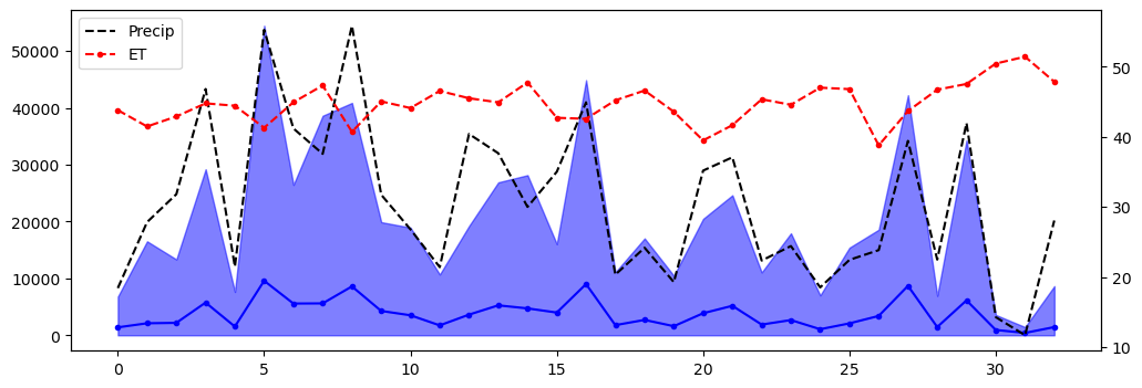
As expected, precipitation amount is the main driver of the yearly discharge regime here
Baseflow separation
Baseflow separation is a method to separate the quick response hydrograph (storm runoff) from the long term flow. We’re going to go back to the complete daily dataset to perform this operation. The following cell contains a low pass filtration method that is used for digital baseflow separation. We’ll use these in our analysis
[40]:
def _baseflow_low_pass_filter(arr, beta, enforce):
    """
    Private method to apply digital baseflow separation filter
    (Lyne & Hollick, 1979; Nathan & Mcmahon, 1990;
    Boughton, 1993; Chapman & Maxwell, 1996).

    This method should not be called by the user!

    Method removes "spikes" which would be consistent with storm flow
    events from data.

    Parameters
    ----------
    arr : np.array
        streamflow or municipal pumping time series

    beta : float
        baseflow filtering parameter that ranges from 0 - 1
        values in 0.8 - 0.95 range used in literature for
        streamflow baseflow separation

    enforce : bool
        enforce physical constraint of baseflow less than measured flow

    Returns
    -------
        np.array of filtered data
    """
    # prepend 10 records to data for initial spin up
    # these records will be dropped before returning data to user
    qt = np.zeros((arr.size + 10,), dtype=float)
    qt[0:10] = arr[0:10]
    qt[10:] = arr[:]

    qdt = np.zeros((arr.size + 10,), dtype=float)
    qbf = np.zeros((arr.size + 10,), dtype=float)

    y = (1. + beta) / 2.

    for ix in range(qdt.size):
        if ix == 0:
            qbf[ix] = qt[ix]
            continue

        x = beta * qdt[ix - 1]
        z = qt[ix] - qt[ix - 1]
        qdt[ix] = x + (y * z)

        qb = qt[ix] - qdt[ix]
        if enforce:
            if qb > qt[ix]:
                qbf[ix] = qt[ix]
            else:
                qbf[ix] = qb

        else:
            qbf[ix] = qb

    return qbf[10:]


def baseflow_low_pass_filter(arr, beta=0.9, T=1, enforce=True):
    """
    User method to apply digital baseflow separation filter
    (Lyne & Hollick, 1979; Nathan & Mcmahon, 1990;
    Boughton, 1993; Chapman & Maxwell, 1996).

    Method removes "spikes" which would be consistent with storm flow
    events from data.

    Parameters
    ----------
    arr : np.array
        streamflow or municipal pumping time series

    beta : float
        baseflow filtering parameter that ranges from 0 - 1
        values in 0.8 - 0.95 range used in literature for
        streamflow baseflow separation

    T : int
        number of recursive filtering passes to apply to the data

    enforce : bool
        enforce physical constraint of baseflow less than measured flow

    Returns
    -------
        np.array of baseflow
    """
    for _ in range(T):
        arr = _baseflow_low_pass_filter(arr, beta, enforce)

    return arr
Class exercise 4: baseflow separation
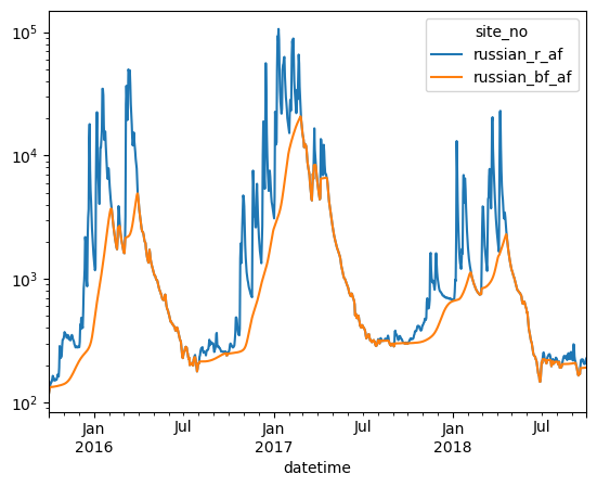
Using the full dataframe discharge dataframe, df2, get the baseflows for the Russian River (in acre-ft) and add these to the dataframe as a new column named russian_bf_af.
The function baseflow_low_pass_filter() will be used to perform baseflow. This function takes a numpy array of stream discharge and runs a digital low pass filtration method to calculate baseflow.
After performing baseflow separation plot both the baseflow and the total discharge for the years 2015 - 2017.
Hints:
make sure to use the
.valuesproperty when you get discharge data from the pandas dataframefeel free to play with the input parameters
betaandT.betais commonly between 0.8 - 0.95 for hydrologic problems.Tis the number of filter passes over the data, therefore increasingTwill create a smoother profile. I recommend starting with aTvalue of around 5 and adjusting it to see how it changes the baseflow profile.
[41]:
baseflow = baseflow_low_pass_filter(df2["russian_r_af"].values, beta=0.90, T=5)
df2["russian_bf_af"] = baseflow

fig = plt.figure(figsize=(15, 10))
tdf = df2[(df2.year >= 2015) & (df2.year <= 2017)]
ax = tdf[["russian_r_af", "russian_bf_af"]].plot()
ax.set_yscale("log");
<Figure size 1500x1000 with 0 Axes>
Looking at trends and seasonal cycles in the data with statsmodels
statsmodels is a Python module that provides classes and functions for the estimation of many different statistical models, as well as for conducting statistical tests, and statistical data exploration. For more information on statsmodels and it’s many features visit the getting started guide
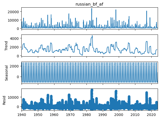
For this example we’ll be using time series analysis to perform a seasonal decomposition using moving averages. The statsmodels function seasonal_decompose will perform this analysis and return the data trend, seasonal fluctuations, and residuals.
[42]:
df2["russian_bf_af"] = baseflow_low_pass_filter(df2["russian_r_af"].values, beta=0.9, T=5)
# drop nan values prior to running decomposition
dfsm = df2[df2['russian_bf_af'].notna()]

dfsm.head()
# decompose
decomposition = sm.tsa.seasonal_decompose(dfsm["russian_bf_af"], period=365, model="additive")

decomposition.plot()
mpl.rcParams['figure.figsize'] = [14, 14];
Now let’s plot our baseflow trend against the baseflow we calculated
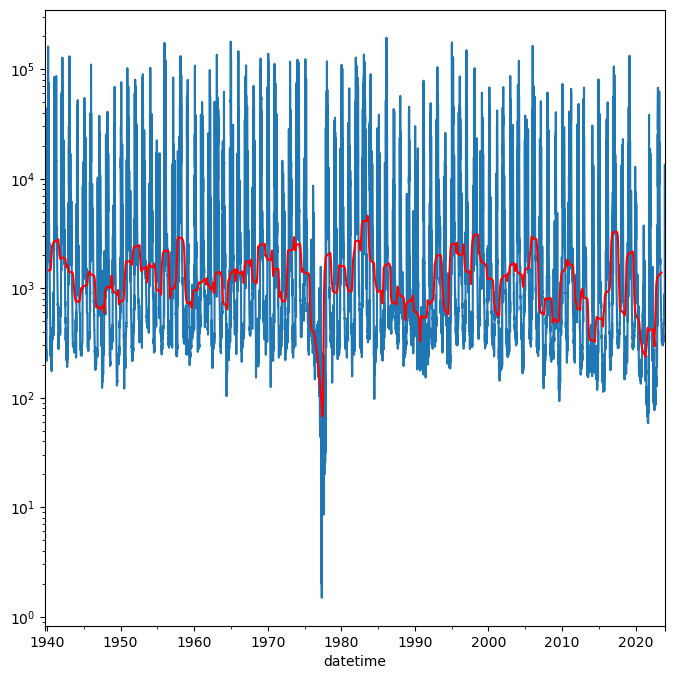
[43]:
fig, ax = plt.subplots(figsize=(8, 8))

ax = df2["russian_r_af"].plot(ax=ax)
ax.plot(decomposition.trend.index, decomposition.trend, "r-", lw=1.5)
ax.set_yscale('log')
plt.savefig("russian_river.png")
/tmp/ipykernel_10575/1871956059.py:4: UserWarning: This axis already has a converter set and is updating to a potentially incompatible converter
  ax.plot(decomposition.trend.index, decomposition.trend, "r-", lw=1.5)
What’s going on at the end of the 1970’s? Why is the baseflow trend so low and peak flows are also low?
From “California’s Most Significant Droughts”, Chapter 3
The setting for the 1976-77 drought differed significantly from the dry times of the 1920s-30s. Although only a two-year event, its hydrology was severe. Based on 114 years of computed statewide runoff, 1977 occupies rank 114 (driest year) and 1976 is in rank 104. The drought was notable for the impacts experienced by water agencies that were unprepared for such conditions. One reason for the lack of preparedness was the perception of relatively ample water supplies in most areas of the state.
We can also see the analysis that there is an overall reduction in baseflow from 1940’s to the 2020’s
Writing yearly plots of data to a PDF document
We can write the plots we make with pandas to a multipage pdf using matplotlib’s PdfPages. For this example we’ll make yearly plots of all of the discharge, baseflow, and baseflow trend and bundle them into a single pdf document.
[44]:
# add the decomposition trend to the dataframe to make plotting easy
df2["baseflow_trend"] = decomposition.trend

pdf_file = data_path / "all_years_russian.pdf"
with PdfPages(pdf_file) as outpdf:
    for year in sorted(df2.year.unique()):
        plt.figure()
        tdf = df2[df2.year == year]
        tdf[["russian_r_af", "russian_bf_af", "baseflow_trend"]].plot()
        plt.xlabel("date")
        plt.ylabel("acre-feet")
        plt.ylim([1, 300000])
        plt.yscale("log")
        plt.tight_layout()
        outpdf.savefig()
        plt.close('all')
Go into the “data/pandas” and open up the file “all_years_russian.pdf” to check out the plots.
Back to the basics:
Now that we’ve done some analysis on real data, let’s go back to the basic and briefly discuss how to adjust data values in pandas
Adjusting a whole column of data values
Because pandas series objects (columns) are built off of numpy, we can perform mathematical operations in place on a whole column similarly to numpy arrays
[45]:
df3 = df2.copy()
# Adding values
df3["russian_r"] += 10000

# Subtracting values
df3["russian_r"] -= 10000

# multiplication
df3["russian_r"] *= 5

# division
df3["russian_r"] /= 5

# more complex operations
df3["russian_r"] = np.log10(df3["russian_r"].values)
df3.head()
[45]:
| site_no | russian_r | austin_c | year | russian_r_cfd | russian_r_af | austin_c_cfd | austin_c_af | day_of_year | russian_bf_af | baseflow_trend |
|---|---|---|---|---|---|---|---|---|---|---|
| datetime | ||||||||||
| 1939-10-01 00:00:00+00:00 | 2.267172 | NaN | 1939 | 15984000.0 | 366.942991 | NaN | NaN | 274 | 366.942991 | NaN |
| 1939-10-02 00:00:00+00:00 | 2.267172 | NaN | 1939 | 15984000.0 | 366.942991 | NaN | NaN | 275 | 366.942991 | NaN |
| 1939-10-03 00:00:00+00:00 | 2.267172 | NaN | 1939 | 15984000.0 | 366.942991 | NaN | NaN | 276 | 366.942991 | NaN |
| 1939-10-04 00:00:00+00:00 | 2.267172 | NaN | 1939 | 15984000.0 | 366.942991 | NaN | NaN | 277 | 366.942991 | NaN |
| 1939-10-05 00:00:00+00:00 | 2.267172 | NaN | 1939 | 15984000.0 | 366.942991 | NaN | NaN | 278 | 366.942991 | NaN |
updating values by position
We can update single or multiple values by their position in the dataframe using .iloc
[46]:
df3.iloc[0, 1] = 999
df3.head()
[46]:
| site_no | russian_r | austin_c | year | russian_r_cfd | russian_r_af | austin_c_cfd | austin_c_af | day_of_year | russian_bf_af | baseflow_trend |
|---|---|---|---|---|---|---|---|---|---|---|
| datetime | ||||||||||
| 1939-10-01 00:00:00+00:00 | 2.267172 | 999.0 | 1939 | 15984000.0 | 366.942991 | NaN | NaN | 274 | 366.942991 | NaN |
| 1939-10-02 00:00:00+00:00 | 2.267172 | NaN | 1939 | 15984000.0 | 366.942991 | NaN | NaN | 275 | 366.942991 | NaN |
| 1939-10-03 00:00:00+00:00 | 2.267172 | NaN | 1939 | 15984000.0 | 366.942991 | NaN | NaN | 276 | 366.942991 | NaN |
| 1939-10-04 00:00:00+00:00 | 2.267172 | NaN | 1939 | 15984000.0 | 366.942991 | NaN | NaN | 277 | 366.942991 | NaN |
| 1939-10-05 00:00:00+00:00 | 2.267172 | NaN | 1939 | 15984000.0 | 366.942991 | NaN | NaN | 278 | 366.942991 | NaN |
updating values based on location
We can update values in the dataframe based on their index and column headers too using .loc
[47]:
df3.loc[df3.index[0], 'russian_r'] *= 100
df3.head()
[47]:
| site_no | russian_r | austin_c | year | russian_r_cfd | russian_r_af | austin_c_cfd | austin_c_af | day_of_year | russian_bf_af | baseflow_trend |
|---|---|---|---|---|---|---|---|---|---|---|
| datetime | ||||||||||
| 1939-10-01 00:00:00+00:00 | 226.717173 | 999.0 | 1939 | 15984000.0 | 366.942991 | NaN | NaN | 274 | 366.942991 | NaN |
| 1939-10-02 00:00:00+00:00 | 2.267172 | NaN | 1939 | 15984000.0 | 366.942991 | NaN | NaN | 275 | 366.942991 | NaN |
| 1939-10-03 00:00:00+00:00 | 2.267172 | NaN | 1939 | 15984000.0 | 366.942991 | NaN | NaN | 276 | 366.942991 | NaN |
| 1939-10-04 00:00:00+00:00 | 2.267172 | NaN | 1939 | 15984000.0 | 366.942991 | NaN | NaN | 277 | 366.942991 | NaN |
| 1939-10-05 00:00:00+00:00 | 2.267172 | NaN | 1939 | 15984000.0 | 366.942991 | NaN | NaN | 278 | 366.942991 | NaN |
Class exercise 5: setting data
The russian river discharge in cubic feet per day highly variable and represented by large numbers. To make this data easier to read and plot, update it to a log10 representation.
Then use either a location based method to change the value in austin_c on 10-4-1939 to 0.
Finally display the first 5 records in the notebook.
[48]:
df3["russian_r_cfd"] = np.log10(df3["russian_r_cfd"])
df3.loc[df3.index[3], "austin_c"] = 0
df3.head()
[48]:
| site_no | russian_r | austin_c | year | russian_r_cfd | russian_r_af | austin_c_cfd | austin_c_af | day_of_year | russian_bf_af | baseflow_trend |
|---|---|---|---|---|---|---|---|---|---|---|
| datetime | ||||||||||
| 1939-10-01 00:00:00+00:00 | 226.717173 | 999.0 | 1939 | 7.203685 | 366.942991 | NaN | NaN | 274 | 366.942991 | NaN |
| 1939-10-02 00:00:00+00:00 | 2.267172 | NaN | 1939 | 7.203685 | 366.942991 | NaN | NaN | 275 | 366.942991 | NaN |
| 1939-10-03 00:00:00+00:00 | 2.267172 | NaN | 1939 | 7.203685 | 366.942991 | NaN | NaN | 276 | 366.942991 | NaN |
| 1939-10-04 00:00:00+00:00 | 2.267172 | 0.0 | 1939 | 7.203685 | 366.942991 | NaN | NaN | 277 | 366.942991 | NaN |
| 1939-10-05 00:00:00+00:00 | 2.267172 | NaN | 1939 | 7.203685 | 366.942991 | NaN | NaN | 278 | 366.942991 | NaN |
Now for some powerful analysis using fourier analysis to extract the data’s signal.
Some background for your evening viewing: https://youtu.be/spUNpyF58BY
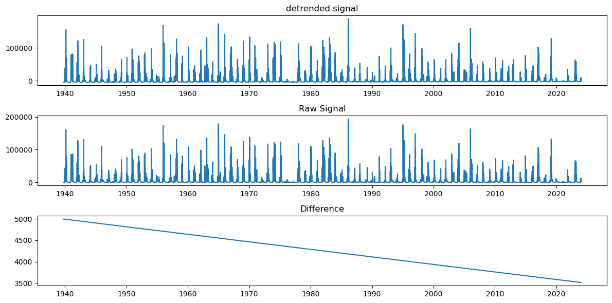
We have to detrend the data for fast fourier transforms to work properly. Here’s a discussion on why:
https://groups.google.com/forum/#!topic/comp.dsp/kYDZqetr_TU
Fortunately we can easily do this in python using scipy!
https://docs.scipy.org/doc/scipy/reference/generated/scipy.signal.detrend.html
Let’s create a new dataframe with only the data we’re interested in analysing.
[49]:
df_data = df2[["russian_r_af", "year"]]
df_data = df_data.rename(columns={"russian_r_af": "Q"})
df_data.describe()
[49]:
| site_no | Q | year |
|---|---|---|
| count | 30773.000000 | 30773.000000 |
| mean | 4254.981092 | 1980.626036 |
| std | 11328.372092 | 24.322069 |
| min | 1.487607 | 1939.000000 |
| 25% | 345.124759 | 1960.000000 |
| 50% | 672.398238 | 1981.000000 |
| 75% | 2657.857341 | 2002.000000 |
| max | 193785.568837 | 2023.000000 |
But first let’s also set the water year by date on this dataframe and drop the single nan value from the dataframe
[50]:
df_data['water_year'] = df_data.index.shift(30+31+31,freq='d').year
df_data.dropna(inplace=True)
df_data["detrended"] = detrend(df_data.Q.values)
/tmp/ipykernel_10575/608845639.py:1: Pandas4Warning: 'd' is deprecated and will be removed in a future version, please use 'D' instead.
  df_data['water_year'] = df_data.index.shift(30+31+31,freq='d').year
[51]:
fig = plt.figure(figsize=(12,6))
ax = plt.subplot(3,1,1)
plt.plot(df_data.detrended)
plt.title('detrended signal')

plt.subplot(3,1,2)
plt.plot(df_data.index, df_data.Q)
plt.title('Raw Signal')

plt.subplot(3,1,3)
plt.plot(df_data.index, df_data.Q - df_data.detrended)
plt.title('Difference')

plt.tight_layout()
Evaluate and plot the Period Spectrum to see timing of recurrence
Here we’ve created a function that performs fast fourier transforms and then plot’s the spectrum for signals of various lengths.
[52]:
def fft_and_plot(df, plot_dominant_periods=4):
    N = len(df)
    yf = np.fft.fft(df.detrended)
    yf = np.abs(yf[:int(N / 2)])

    # get the right frequency
    # https://docs.scipy.org/doc/numpy/reference/generated/numpy.fft.fftfreq.html#numpy.fft.fftfreq
    d = 1. # day
    f = np.fft.fftfreq(N, d)[:int(N/2)]
    f[0] = .00001
    per = 1./f # days

    fig = plt.figure(figsize=(12,6))
    ax = plt.subplot(2,1,1)
    plt.plot(per, yf)
    plt.xscale('log')

    top=np.argsort(yf)[-plot_dominant_periods:]
    j=(10-plot_dominant_periods)/10
    for i in top:
        plt.plot([per[i], per[i]], [0,np.max(yf)], 'r:')
        plt.text(per[i], j*np.max(yf), f"{per[i] :.2f}")
        j+=0.1

    plt.title('Period Spectrum')
    plt.grid()
    ax.set_xlabel('Period (days)')
    plt.xlim([1, 1e4])

    plt.subplot(2,1,2)
    plt.plot(df.index,df.Q)
    plt.title('Raw Signal')
    plt.tight_layout()
Now let’s look at the whole signal
[53]:
fft_and_plot(df_data)
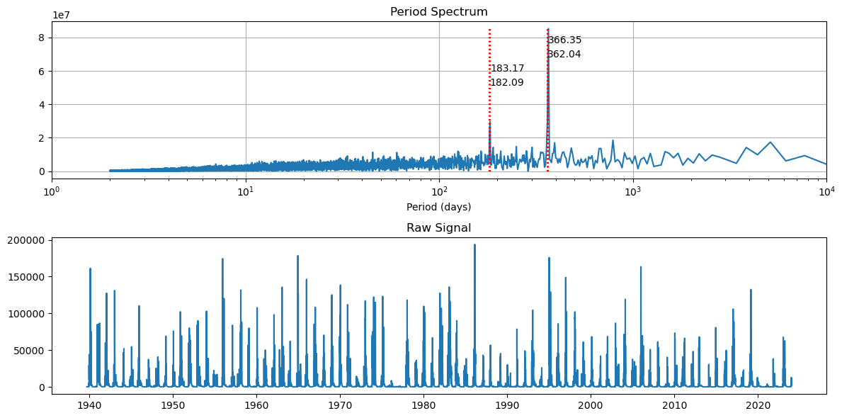
We see a strong annual frequency that corresponds to spring snowmelt from the surrounding mountain ranges. The second strongest frequency is biannually, and is likely due to the onset of fall in winter rains
Okay, what about years before dams were installed on the Russian River.
Let’s get in the wayback machine and look at only the years prior to 1954!
[54]:
fft_and_plot(df_data[df_data.index.year < 1954])
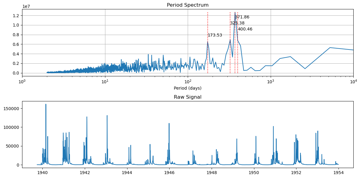
The binanual and annual signals have a much wider spread, which suggests that peak runoff was a little more variable in it’s timing compared to the entire data record.
What if we focus in on after 1954?
[55]:
fft_and_plot(df_data[(df_data.index.year > 1954)])
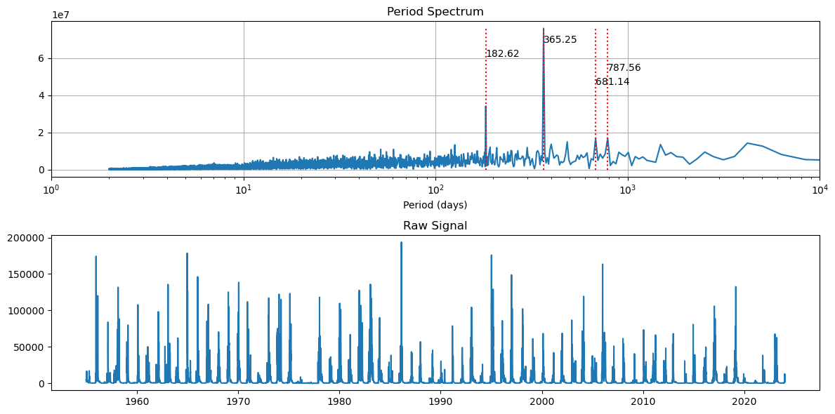
It looks like flows are more controlled with a tighter periods.
So post dam construction, flows are much more controlled with regular release schedules.