09: Demonstration of MODFLOW 6 Groundwater Transport with a Voronoi Grid
MODFLOW 6 includes a Groundwater Transport (GWT) Model for simulation of solute transport through the subsurface. The GWT Model can be used with structured or unstructured model grids. The purpose of this example is to demonstrate the construction, running, and post-processing of a simple solute transport model.
The solute transport model is based on an existing flow model of the Freyberg example. The flow model uses a voronoi model grid to simulate steady-state conditions. In this notebook, we create a transient solute transport model using the same voronoi grid.
The following steps are taken in this notebook:
Load the existing flow model into FloPy
Plot the model grid
Create the solute transport model
Run the solute transport model with MODFLOW 6
Create animations of the model results
Imports
[1]:
import warnings
import numpy as np
import matplotlib.pyplot as plt
import matplotlib.colors as colors
import flopy
from flopy.utils.triangle import Triangle as Triangle
Load and Plot the Existing Flow Model
[2]:
model_ws_load = "./data/voronoi/"
model_ws = "./temp/voronoi-gwt/"
name = "voronoi"
name_load = "project"
Load a few shapefiles with geopandas
[3]:
river_shp = "data_project/Flowline_river.shp"
wells_shp = "data_project/pumping_well_locations.shp"
Load the existing voronoi groundwater flow model
[4]:
%%capture
sim = flopy.mf6.MFSimulation.load(sim_ws=model_ws_load, sim_name=name)
Get the gwf model
[5]:
gwf = sim.get_model()
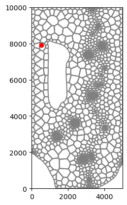
We will assign a constant concentration condition to the x, y location of 550, 7900. Use the modelgrid.intersect method to determine the cell number for the constant concentration condition.
[6]:
x, y = 550, 7900
[7]:
cc_cell = gwf.modelgrid.intersect(x, y)
cc_cell
[7]:
2027
Plot the grid
[8]:
gwf.modelgrid.plot()
ax = plt.gca()
ax.plot(x, y, marker="o", lw=0, color="red", )
[8]:
[<matplotlib.lines.Line2D at 0x7f59da479be0>]
Create the Groundwater Transport Model
Get data from the GWF DISV package
[9]:
nlay, ncpl = gwf.disv.nlay.array, gwf.disv.ncpl.array
nlay, ncpl
[9]:
(3, 2240)
[10]:
top, botm = gwf.disv.top.array, gwf.disv.botm.array
top.shape, botm.shape
[10]:
((2240,), (3, 2240))
[11]:
nverts = gwf.disv.nvert.array
nverts
[11]:
4908
[12]:
vertices, cell2d = gwf.disv.vertices.array, gwf.disv.cell2d.array
Create the GWT model
[13]:
sim_gwt = flopy.mf6.MFSimulation(sim_name=name, sim_ws=model_ws)
tdis = flopy.mf6.ModflowTdis(sim_gwt,
time_units="days",
perioddata=((10000.0, 100, 1.0),),
)
ims = flopy.mf6.ModflowIms(
sim_gwt,
linear_acceleration="bicgstab",
outer_maximum=200,
inner_maximum=100,
print_option="all",
)
[14]:
gwt = flopy.mf6.ModflowGwt(sim_gwt, modelname=name)
Create the GWT packages
[15]:
dis = flopy.mf6.ModflowGwtdisv(
gwt,
length_units="feet",
nlay=nlay,
ncpl=ncpl,
nvert=nverts,
top=top,
botm=botm,
vertices=vertices,
cell2d=cell2d,
)
ic = flopy.mf6.ModflowGwtic(gwt, strt=0.0)
# use the TVD advection solver scheme, upstream is default
adv = flopy.mf6.ModflowGwtadv(gwt, scheme="tvd")
# define logitudinal and transverse dispersivity
dsp = flopy.mf6.ModflowGwtdsp(gwt, alh=50.0, ath1=5)
# define a uniform porosity in the "mobile" portion of the aquifer
mst = flopy.mf6.ModflowGwtmst(gwt, porosity=0.2)
# point the transport model to the flow model head and budget outputs
# these must include outputs from ALL time steps
pd = [
("GWFHEAD", f"../../{model_ws_load}{name_load}.hds", None),
("GWFBUDGET", f"../../{model_ws_load}{name_load}.cbc", None),
]
fmi = flopy.mf6.ModflowGwtfmi(gwt, packagedata=pd)
ssm = flopy.mf6.ModflowGwtssm(gwt)
# this is where we define the constanc concentration
cnc = flopy.mf6.ModflowGwtcnc(gwt, stress_period_data=[(0, cc_cell, 100.)])
oc = flopy.mf6.ModflowGwtoc(
gwt,
concentration_filerecord=f"{name}.ucn",
saverecord=[("CONCENTRATION", "ALL"),],
printrecord=[("BUDGET", "ALL")],
)
# write the model datasets
sim_gwt.write_simulation()
writing simulation...
writing simulation name file...
writing simulation tdis package...
writing solution package ims_-1...
writing model voronoi...
writing model name file...
writing package disv...
writing package ic...
writing package adv...
writing package dsp...
writing package mst...
writing package fmi...
writing package ssm...
writing package cnc_0...
INFORMATION: maxbound in ('gwt6', 'cnc', 'dimensions') changed to 1 based on size of stress_period_data
writing package oc...
Run the Solute Transport Model
[16]:
sim_gwt.run_simulation()
FloPy is using the following executable to run the model: ../../../../../../../../../.local/bin/mf6
MODFLOW 6
U.S. GEOLOGICAL SURVEY MODULAR HYDROLOGIC MODEL
VERSION 6.7.0 02/05/2026
MODFLOW 6 compiled Feb 05 2026 22:38:38 with Intel(R) Fortran Intel(R) 64
Compiler Classic for applications running on Intel(R) 64, Version 2021.6.0
Build 20220226_000000
This software has been approved for release by the U.S. Geological
Survey (USGS). Although the software has been subjected to rigorous
review, the USGS reserves the right to update the software as needed
pursuant to further analysis and review. No warranty, expressed or
implied, is made by the USGS or the U.S. Government as to the
functionality of the software and related material nor shall the
fact of release constitute any such warranty. Furthermore, the
software is released on condition that neither the USGS nor the U.S.
Government shall be held liable for any damages resulting from its
authorized or unauthorized use. Also refer to the USGS Water
Resources Software User Rights Notice for complete use, copyright,
and distribution information.
MODFLOW runs in SEQUENTIAL mode
Run start date and time (yyyy/mm/dd hh:mm:ss): 2026/07/19 16:29:17
Writing simulation list file: mfsim.lst
Using Simulation name file: mfsim.nam
Solving: Stress period: 1 Time step: 1
Solving: Stress period: 1 Time step: 2
Solving: Stress period: 1 Time step: 3
Solving: Stress period: 1 Time step: 4
Solving: Stress period: 1 Time step: 5
Solving: Stress period: 1 Time step: 6
Solving: Stress period: 1 Time step: 7
Solving: Stress period: 1 Time step: 8
Solving: Stress period: 1 Time step: 9
Solving: Stress period: 1 Time step: 10
Solving: Stress period: 1 Time step: 11
Solving: Stress period: 1 Time step: 12
Solving: Stress period: 1 Time step: 13
Solving: Stress period: 1 Time step: 14
Solving: Stress period: 1 Time step: 15
Solving: Stress period: 1 Time step: 16
Solving: Stress period: 1 Time step: 17
Solving: Stress period: 1 Time step: 18
Solving: Stress period: 1 Time step: 19
Solving: Stress period: 1 Time step: 20
Solving: Stress period: 1 Time step: 21
Solving: Stress period: 1 Time step: 22
Solving: Stress period: 1 Time step: 23
Solving: Stress period: 1 Time step: 24
Solving: Stress period: 1 Time step: 25
Solving: Stress period: 1 Time step: 26
Solving: Stress period: 1 Time step: 27
Solving: Stress period: 1 Time step: 28
Solving: Stress period: 1 Time step: 29
Solving: Stress period: 1 Time step: 30
Solving: Stress period: 1 Time step: 31
Solving: Stress period: 1 Time step: 32
Solving: Stress period: 1 Time step: 33
Solving: Stress period: 1 Time step: 34
Solving: Stress period: 1 Time step: 35
Solving: Stress period: 1 Time step: 36
Solving: Stress period: 1 Time step: 37
Solving: Stress period: 1 Time step: 38
Solving: Stress period: 1 Time step: 39
Solving: Stress period: 1 Time step: 40
Solving: Stress period: 1 Time step: 41
Solving: Stress period: 1 Time step: 42
Solving: Stress period: 1 Time step: 43
Solving: Stress period: 1 Time step: 44
Solving: Stress period: 1 Time step: 45
Solving: Stress period: 1 Time step: 46
Solving: Stress period: 1 Time step: 47
Solving: Stress period: 1 Time step: 48
Solving: Stress period: 1 Time step: 49
Solving: Stress period: 1 Time step: 50
Solving: Stress period: 1 Time step: 51
Solving: Stress period: 1 Time step: 52
Solving: Stress period: 1 Time step: 53
Solving: Stress period: 1 Time step: 54
Solving: Stress period: 1 Time step: 55
Solving: Stress period: 1 Time step: 56
Solving: Stress period: 1 Time step: 57
Solving: Stress period: 1 Time step: 58
Solving: Stress period: 1 Time step: 59
Solving: Stress period: 1 Time step: 60
Solving: Stress period: 1 Time step: 61
Solving: Stress period: 1 Time step: 62
Solving: Stress period: 1 Time step: 63
Solving: Stress period: 1 Time step: 64
Solving: Stress period: 1 Time step: 65
Solving: Stress period: 1 Time step: 66
Solving: Stress period: 1 Time step: 67
Solving: Stress period: 1 Time step: 68
Solving: Stress period: 1 Time step: 69
Solving: Stress period: 1 Time step: 70
Solving: Stress period: 1 Time step: 71
Solving: Stress period: 1 Time step: 72
Solving: Stress period: 1 Time step: 73
Solving: Stress period: 1 Time step: 74
Solving: Stress period: 1 Time step: 75
Solving: Stress period: 1 Time step: 76
Solving: Stress period: 1 Time step: 77
Solving: Stress period: 1 Time step: 78
Solving: Stress period: 1 Time step: 79
Solving: Stress period: 1 Time step: 80
Solving: Stress period: 1 Time step: 81
Solving: Stress period: 1 Time step: 82
Solving: Stress period: 1 Time step: 83
Solving: Stress period: 1 Time step: 84
Solving: Stress period: 1 Time step: 85
Solving: Stress period: 1 Time step: 86
Solving: Stress period: 1 Time step: 87
Solving: Stress period: 1 Time step: 88
Solving: Stress period: 1 Time step: 89
Solving: Stress period: 1 Time step: 90
Solving: Stress period: 1 Time step: 91
Solving: Stress period: 1 Time step: 92
Solving: Stress period: 1 Time step: 93
Solving: Stress period: 1 Time step: 94
Solving: Stress period: 1 Time step: 95
Solving: Stress period: 1 Time step: 96
Solving: Stress period: 1 Time step: 97
Solving: Stress period: 1 Time step: 98
Solving: Stress period: 1 Time step: 99
Solving: Stress period: 1 Time step: 100
Run end date and time (yyyy/mm/dd hh:mm:ss): 2026/07/19 16:29:27
Elapsed run time: 10.030 Seconds
Normal termination of simulation.
[16]:
(True, [])
Post-process the results
Use gwt.output. method to get the concentrations. Make an animation the concentrations using flopy.plot methods.
[17]:
head = gwf.output.head().get_data()
spdis = gwf.output.budget().get_data(text="DATA-SPDIS")[0]
qx, qy, qz = flopy.utils.postprocessing.get_specific_discharge(
spdis, gwf, head=gwf.output.head().get_data(),
)
/home/runner/micromamba/envs/pyclass-docs/lib/python3.14/site-packages/flopy/utils/postprocessing.py:617: DeprecationWarning: Setting the shape on a NumPy array has been deprecated in NumPy 2.5.
As an alternative, you can create a new view using np.reshape (with copy=False if needed).
head.shape = modelgrid.shape
/home/runner/micromamba/envs/pyclass-docs/lib/python3.14/site-packages/flopy/utils/postprocessing.py:743: DeprecationWarning: Setting the shape on a NumPy array has been deprecated in NumPy 2.5.
As an alternative, you can create a new view using np.reshape (with copy=False if needed).
qx.shape = modelgrid.shape
/home/runner/micromamba/envs/pyclass-docs/lib/python3.14/site-packages/flopy/utils/postprocessing.py:744: DeprecationWarning: Setting the shape on a NumPy array has been deprecated in NumPy 2.5.
As an alternative, you can create a new view using np.reshape (with copy=False if needed).
qy.shape = modelgrid.shape
/home/runner/micromamba/envs/pyclass-docs/lib/python3.14/site-packages/flopy/utils/postprocessing.py:745: DeprecationWarning: Setting the shape on a NumPy array has been deprecated in NumPy 2.5.
As an alternative, you can create a new view using np.reshape (with copy=False if needed).
qz.shape = modelgrid.shape
[18]:
times = gwt.output.concentration().get_times()
[19]:
warnings.filterwarnings("ignore")
fig, ax = plt.subplots(figsize=(4, 6), constrained_layout=True)
ax.set_aspect(1)
ax.set_xlabel(r'x')
ax.set_ylabel(r'y')
title = ax.set_title(f"Time = {times[0]} days")
# plot persistent items
vmin, vmax = 1e-3, 100.
norm = colors.LogNorm(vmin=vmin, vmax=vmax)
pmv = flopy.plot.PlotMapView(gwt, ax=ax)
pmv.plot_grid(lw=0.5, color="0.5")
pmv.contour_array(
head,
levels=np.linspace(0, 30, 30),
tri_mask=True,
linestyles="-",
colors="blue",
linewidths=0.5,
)
ca_dict = {
"vmin": vmin,
"vmax": vmax,
"norm": norm,
"masked_values": [0],
}
conc_alldata = gwt.output.concentration().get_alldata()
c = conc_alldata[0]
c[c < vmin] = 0.
cont = pmv.plot_array(c, **ca_dict)
clb = fig.colorbar(
cont,
shrink=0.5,
)
def animate(i):
c = conc_alldata[i].flatten()
c[c < vmin] = 0.
cont.set_array(c)
title = ax.set_title(f"Time = {times[i]} days")
return cont
import matplotlib.animation
ani = matplotlib.animation.FuncAnimation(fig, animate, frames=conc_alldata.shape[0])
plt.close()
from IPython.display import HTML
HTML(ani.to_jshtml())
# can use this command to write animation to file
#ani.save("voronoi-conc-animation.avi")
[19]: