
02: Building and post-processing a MODFLOW 6 model
A MODFLOW 6 model will be developed of the domain shown above. This model simulation is based on example 1 in Pollock, D.W., 2016, User guide for MODPATH Version 7—A particle-tracking model for MODFLOW: U.S. Geological Survey Open-File Report 2016–1086, 35 p., http://dx.doi.org/10.3133/ofr20161086.
The model domain will be discretized into 3 layers, 21 rows, and 20 columns. A constant value of 500 ft will be specified for delr and delc. The top (TOP) of the model should be set to 400 ft and the bottom of the three layers should be set to 220 ft, 200 ft, and 0 ft, respectively. The model has one steady-state stress period.
[1]:
import numpy as np
import matplotlib as mpl
import matplotlib.pyplot as plt
import flopy
from flopy.plot import styles
Before we get started lets install MODFLOW 6, other MODFLOW-based executables (MODFLOW-2005, MT3DMS, etc.), and utilities programs used by FloPy (gridgen and triangle) in the Miniforge class environment (pyclass) using FloPy get-modflow functionality (flopy.utils.get_modflow()). Remember that Shift-Tab can be used to see the docstrings for a Python function, method, or function. Press Shift-Tab after the opening parenthesis in flopy.utils.get_modflow() below to see
the docstrings for the function and determine the required (args) and optional arguments (kwaargs).
[2]:
# flopy.utils.get_modflow(":python")
Before creating any of the MODFLOW 6 FloPy objects you should define the simulation workspace (ws) where the model files are and the simulation name (name). The ws should be set to 'data/ex01b' and name should be set to ex01b.
[3]:
ws = "../temp/ex01b"
name = "ex01b"
Create a simulation object, a temporal discretization object, and a iterative model solution object using flopy.mf6.MFSimulation(), flopy.mf6.ModflowTdis(), and flopy.mf6.ModflowIms(), respectively. Set the sim_name to name and sim_ws to ws in the simulation object. Use default values for all temporal discretization and iterative model solution variables. Make sure to include the simulation object (sim) as the first variable in the temporal discretization and
iterative model solution objects.
[4]:
# create simulation (sim = flopy.mf6.MFSimulation())
sim = flopy.mf6.MFSimulation(sim_name=name, sim_ws=ws)

# create tdis package (tdis = flopy.mf6.ModflowTdis(sim))
tdis = flopy.mf6.ModflowTdis(sim)

# create iterative model solution (ims = flopy.mf6.ModflowIms(sim))
ims = flopy.mf6.ModflowIms(sim)
Create the groundwater flow model object (gwf) using flopy.mf6.ModflowGwf(). Make sure to include the simulation object (sim) as the first variable in the groundwater flow model object and set modelname to name. Use Shift-Tab to see the optional variables that can be specified.
[5]:
gwf = flopy.mf6.ModflowGwf(sim, modelname=name)
Create the discretization package using flopy.mf6.ModflowGwfdis(). Use Shift-Tab to see the optional variables that can be specified. A description of the data required by the DIS package (flopy.mf6.ModflowGwfdis()) can be found in the MODFLOW 6 ReadTheDocs document.
FloPy can accommodate all of the options for specifying array data for a model. CONSTANT values for a variable can be specified by using a float or int python variable (as is done below for DELR, DELC, and TOP). LAYERED data can be specified by using a list or CONSTANT values for each layer (as is done below for BOTM data) or a list of numpy arrays or lists. Three-Dimensional data can be specified using a three-dimensional numpy array (with a shape of
(nlay, nrow, ncol)) for this example. More information on how to specify array data can be found in the FloPy ReadTheDocs.
[6]:
nlay, nrow, ncol = 3, 21, 20
delr = delc = 500.0
top = 400.0
botm = [220, 200, 0]
[7]:
dis = flopy.mf6.ModflowGwfdis(
    gwf,
    nlay=nlay,
    nrow=nrow,
    ncol=ncol,
    delr=delr,
    delc=delc,
    top=top,
    botm=botm,
)
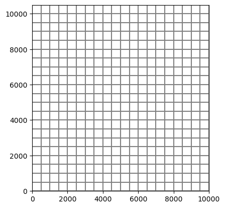
flopy.plot.PlotMapView() and flopy.plot.PlotCrossSection() can be used to confirm that the discretization is correctly defined.
[8]:
mm = flopy.plot.PlotMapView(model=gwf)
mm.plot_grid()
[8]:
<matplotlib.collections.LineCollection at 0x174c2ec30>
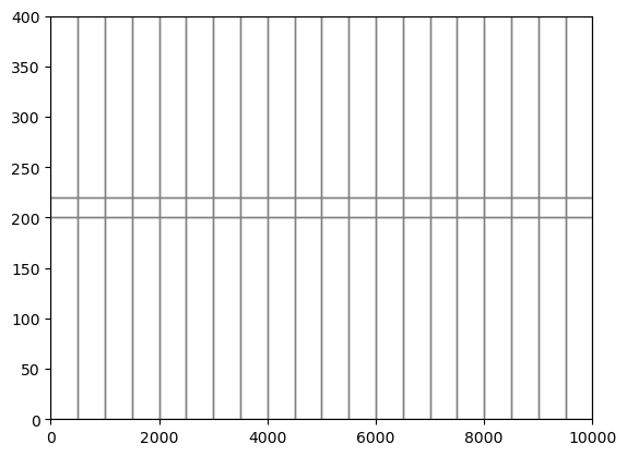
[9]:
xs = flopy.plot.PlotCrossSection(model=gwf, line={"row": 10})
xs.plot_grid()
[9]:
<matplotlib.collections.PatchCollection at 0x174c53a40>
Create the initial conditions (IC) package
Create the initial conditions package (IC) using flopy.mf6.ModflowGwfic() and set the initial head (strt) to 320. Default values can be used for the rest of the initial conditions package input. Use Shift-Tab to see the optional variables that can be specified. A description of the data required by the IC package (flopy.mf6.ModflowGwfic()) can be found in the MODFLOW 6 ReadTheDocs document.
[10]:
ic = flopy.mf6.ModflowGwfic(gwf, strt=320.0)
Create the node property flow (NPF) package
The hydraulic properties for the model are defined in the image above and are specified in the node property flow package (NPF) using flopy.mf6.ModflowGwfnpf(). The first layer should be convertible (unconfined) and the remaining two layers will be non-convertible so icelltype should be [1, 0, 0]. The variable save_specific_discharge should be set to True so that specific discharge data are saved to the cell-by-cell file and can be used to plot discharge. Use
Shift-Tab to see the optional variables that can be specified. A description of the data required by the NPF package (flopy.mf6.ModflowGwfic()) can be found in the MODFLOW 6 ReadTheDocs document.
[11]:
kh = [50, 0.01, 200]
kv = [10, 0.01, 20]
icelltype = [1, 0, 0]
[12]:
npf = flopy.mf6.ModflowGwfnpf(
    gwf, save_specific_discharge=True, icelltype=icelltype, k=kh, k33=kv
)
Create the recharge package
The recharge rate is defined in the image above. Use the flopy.mf6.ModflowGwfrcha() method to specify recharge data using arrays. Use Shift-Tab to see the optional variables that can be specified. A description of the data required by the RCH package (flopy.mf6.ModflowGwfrcha()) can be found in the MODFLOW 6 ReadTheDocs document.
[13]:
rch = flopy.mf6.ModflowGwfrcha(gwf, recharge=0.005)
Create the well package
The well is located in layer 3, row 11, column 10. The pumping rate is defined in the image above. Use the flopy.mf6.ModflowGwfwel() method to specify well data for the well package (WEL). Use Shift-Tab to see the optional variables that can be specified. A description of the data required by the WEL package (flopy.mf6.ModflowGwfwel()) can be found in the MODFLOW 6 ReadTheDocs document.
stress_period_data for list-based stress packages (for example, WEL, DRN, RIV, and GHB) is specified as a dictionary with the zero-based stress-period number as the key and a list of tuples, with the tuple containing the data required for each stress entry. For example, each tuple for the WEL package includes a zero-based cellid and the well rate (cellid, q). For this example, the zero-based cellid for WEL package can be a tuple with the (layer, row, column)
for the well or three integers separated by a comma layer, row, column. More information on how to specify stress_period_data for list based stress packages can be found in the FloPy ReadTheDocs.
An example of a stress_period_data tuple for the WEL package is
# (layer, row, column, q)
(0, 0, 0, -1e5)
[14]:
wel_spd = {0: [[(2, 10, 9), -150000]]}
wel = flopy.mf6.ModflowGwfwel(
    gwf, print_input=True, stress_period_data=wel_spd
)
Create the river package
The river is located in layer 1 and column 20 in every row in the model. The river stage stage and bottom are at 320 and 318, respectively; the river conductance is 1e5. Use the flopy.mf6.ModflowGwfriv() method to specify well data for the river package (RIV). Use Shift-Tab to see the optional variables that can be specified. A description of the data required by the RIV package (flopy.mf6.ModflowGwfriv()) can be found in the MODFLOW 6 ReadTheDocs
document.
An example of a stress_period_data tuple for the RIV package is
# (layer, row, column, stage, cond, rbot)
(0, 0, 0, 320., 1e5, 318.)
HINT: list comprehension is an easy way to create a river cell in every row in column 20 of the model.
[15]:
riv_spd = {0: [((0, i, 19), 320, 1e5, 318) for i in range(nrow)]}
riv_spd
[15]:
{0: [((0, 0, 19), 320, 100000.0, 318),
  ((0, 1, 19), 320, 100000.0, 318),
  ((0, 2, 19), 320, 100000.0, 318),
  ((0, 3, 19), 320, 100000.0, 318),
  ((0, 4, 19), 320, 100000.0, 318),
  ((0, 5, 19), 320, 100000.0, 318),
  ((0, 6, 19), 320, 100000.0, 318),
  ((0, 7, 19), 320, 100000.0, 318),
  ((0, 8, 19), 320, 100000.0, 318),
  ((0, 9, 19), 320, 100000.0, 318),
  ((0, 10, 19), 320, 100000.0, 318),
  ((0, 11, 19), 320, 100000.0, 318),
  ((0, 12, 19), 320, 100000.0, 318),
  ((0, 13, 19), 320, 100000.0, 318),
  ((0, 14, 19), 320, 100000.0, 318),
  ((0, 15, 19), 320, 100000.0, 318),
  ((0, 16, 19), 320, 100000.0, 318),
  ((0, 17, 19), 320, 100000.0, 318),
  ((0, 18, 19), 320, 100000.0, 318),
  ((0, 19, 19), 320, 100000.0, 318),
  ((0, 20, 19), 320, 100000.0, 318)]}
[16]:
riv = flopy.mf6.ModflowGwfriv(gwf, stress_period_data=riv_spd)
Build output control
Define the output control package (OC) for the model using the flopy.mf6.ModflowGwfoc() method to [('HEAD', 'ALL'), ('BUDGET', 'ALL')] to save the head and flow for the model. Also the head (head_filerecord) and cell-by-cell flow (budget_filerecord) files should be set to f"{name}.hds" and f"{name}.cbc", respectively. Use Shift-Tab to see the optional variables that can be specified. A description of the data required by the OC package
(flopy.mf6.ModflowGwfoc()) can be found in the MODFLOW 6 ReadTheDocs document.
[17]:
hname = f"{name}.hds"
cname = f"{name}.cbc"
oc = flopy.mf6.ModflowGwfoc(
    gwf,
    budget_filerecord=cname,
    head_filerecord=hname,
    saverecord=[("HEAD", "ALL"), ("BUDGET", "ALL")],
)
[ ]:
Because we haven’t set SAVE_FLOWS to True in all of the packages we can set .name_file.save_flows to True for the groundwater flow model (gwf) to save flows for all packages that can save flows.
[18]:
gwf.name_file.save_flows = True
Add head observations
Define observations of head at a couple locations in the model. This is helpful to track continuous output at those locations and will write out CSV files that are easy to process for parameter estimation or other purposes. An observation package is in utilities (OSB) for the model is created using the flopy.mf6.ModflowUtlobs() method. Use Shift-Tab to see the optional variables that can be specified although a key format issue may be missing. A description of the data required by
the OBS package (flopy.mf6.ModflowUtlobs()) can be found in the MODFLOW 6 ReadTheDocs document.
Pro Tip: The continous object must be a dictionary with keys being filenames in which to write the output, and values should be a list of lists with each list representing an observation location including a name, obstype, and cell location. For example ['obswell1','head',(0,4,4)].
[19]:
obs = flopy.mf6.ModflowUtlobs(gwf,
                              digits=6,
                              continuous={("head_obs.csv"): [['obswell1','head',(0,4,4)],
                                                              ['obswell2','head',(2,4,4)]]})
Write the model files and run the model
Write the MODFLOW 6 model files using sim.write_simulation(). Use Shift-Tab to see the optional variables that can be specified for .write_simulation().
[20]:
sim.write_simulation()
writing simulation...
  writing simulation name file...
  writing simulation tdis package...
  writing solution package ims_-1...
  writing model ex01b...
    writing model name file...
    writing package dis...
    writing package ic...
    writing package npf...
    writing package rcha_0...
    writing package wel_0...
INFORMATION: maxbound in ('gwf6', 'wel', 'dimensions') changed to 1 based on size of stress_period_data
    writing package riv_0...
INFORMATION: maxbound in ('gwf6', 'riv', 'dimensions') changed to 21 based on size of stress_period_data
    writing package oc...
    writing package obs_0...
Run the model using sim.run_simulation(), which will run the MODFLOW 6 executable installed in the Miniforge class environment (pyclass) and the MODFLOW 6 model files created with .write_simulation(). Use Shift-Tab to see the optional variables that can be specified for .run_simulation().
[21]:
sim.run_simulation()
FloPy is using the following executable to run the model: ../../../../../../../miniforge3/envs/pyclass/bin/mf6
                                   MODFLOW 6
                U.S. GEOLOGICAL SURVEY MODULAR HYDROLOGIC MODEL
                            VERSION 6.6.2 05/12/2025

        MODFLOW 6 compiled May 24 2025 11:40:20 with GCC version 12.4.0

This software has been approved for release by the U.S. Geological
Survey (USGS). Although the software has been subjected to rigorous
review, the USGS reserves the right to update the software as needed
pursuant to further analysis and review. No warranty, expressed or
implied, is made by the USGS or the U.S. Government as to the
functionality of the software and related material nor shall the
fact of release constitute any such warranty. Furthermore, the
software is released on condition that neither the USGS nor the U.S.
Government shall be held liable for any damages resulting from its
authorized or unauthorized use. Also refer to the USGS Water
Resources Software User Rights Notice for complete use, copyright,
and distribution information.


 MODFLOW runs in SEQUENTIAL mode

 Run start date and time (yyyy/mm/dd hh:mm:ss): 2025/09/25 10:54:13

 Writing simulation list file: mfsim.lst
 Using Simulation name file: mfsim.nam

    Solving:  Stress period:     1    Time step:     1

 Run end date and time (yyyy/mm/dd hh:mm:ss): 2025/09/25 10:54:13
 Elapsed run time:  0.023 Seconds

 Normal termination of simulation.
[21]:
(True, [])
Post-process the results
Load the heads and face flows from the hds and cbc files. The head file can be loaded with the gwf.output.head() method. The cell-by-cell file can be loaded with the gwf.output.budget() method.
Name the heads data hds.
[22]:
hobj = gwf.output.head()
[23]:
hds = hobj.get_data()
[24]:
cobj = gwf.output.budget()
The entries in the cell-by-cell file can be determined with the .list_unique_records() method on the cell budget file object.
[25]:
cobj.list_unique_records()
RECORD           IMETH
----------------------
FLOW-JA-FACE         1
DATA-SPDIS           6
WEL                  6
RIV                  6
RCHA                 6
/Users/mnfienen/miniforge3/envs/pyclass/lib/python3.12/site-packages/flopy/utils/binaryfile/__init__.py:1327: DeprecationWarning: list_unique_records() is deprecated; use headers[["text", "imeth"]].drop_duplicates() instead.
  warnings.warn(
Retrieve the 'DATA-SPDIS' data type from the cell-by-cell file. Name the specific discharge data spd.
Cell-by-cell data is returned as a list so access the data by using spd = gwf.output.budget().get_data(text="DATA-SPDIS")[0].
[26]:
spd = cobj.get_data(text="DATA-SPDIS")[0]
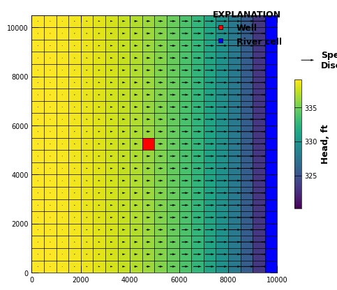
Plot the results
Plot the results using flopy.plot.PlotMapView(). The head results can be plotted using the .plot_array() method. The discharge results can be plotted using the plot_specific_discharge() method. Boundary conditions can be plotted using the .plot_bc() method.
[27]:
with styles.USGSMap():
    mm = flopy.plot.PlotMapView(model=gwf, layer=0, extent=gwf.modelgrid.extent)
    cbv = mm.plot_array(hds)
    q = mm.plot_vector(spd["qx"], spd["qy"])
    mm.plot_bc("RIV", color="blue")
    mm.plot_bc("WEL", plotAll=True)
    mm.plot_grid(lw=0.5, color="black")

    # create data outside of plot limits for legend data
    font_prop = mpl.font_manager.FontProperties(size=9, weight="bold")
    mm.ax.plot(-100, -100, marker="s", lw=0, ms=4, mfc="red", mec="black", mew=0.5, label="Well")
    mm.ax.plot(-100, -100, marker="s", lw=0, ms=4, mfc="blue", mec="black", mew=0.5, label="River cell")

    # plot legend
    styles.graph_legend(bbox_to_anchor=(1.05, 1.05))
    plt.quiverkey(q, X = 1.15, Y = 0.825, U = .200, label ='Specific\nDischarge', labelpos="E", fontproperties=font_prop)

    # plot colorbar
    cb = plt.colorbar(cbv, ax=mm.ax, shrink=0.5)
    cb.set_label(label="Head, ft", weight="bold")
Read in the output from the observation package
[28]:
import pandas as pd
obs_results  = pd.read_csv(ws + '/head_obs.csv')
[29]:
obs_results
[29]:
| time | OBSWELL1 | OBSWELL2 | |
|---|---|---|---|
| 0 | 1.0 | 338.499 | 331.529 |
[ ]: