06: FloPy class project: Structured grid version
[1]:
import numpy as np
import matplotlib.pyplot as plt
import geopandas as gpd
import shapely
import shapefile
import flopy
from flopy.utils.gridgen import Gridgen
from flopy.discretization import StructuredGrid, VertexGrid
from flopy.utils.triangle import Triangle as Triangle
from flopy.utils.voronoi import VoronoiGrid
from flopy.utils.gridintersect import GridIntersect
[2]:
model_ws = "../temp/structured/"
Load a few raster files
[3]:
bottom = flopy.utils.Raster.load("../data_project/aquifer_bottom.asc")
top = flopy.utils.Raster.load("../data_project/aquifer_top.asc")
kaq = flopy.utils.Raster.load("../data_project/aquifer_k.asc")
Load a few shapefiles with geopandas
[4]:
river = gpd.read_file("../data_project/Flowline_river.shp")
inactive = gpd.read_file("../data_project/inactive_area.shp")
active = gpd.read_file("../data_project/active_area.shp")
wells = gpd.read_file("../data_project/pumping_well_locations.shp")
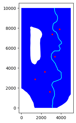
Plot the shapefiles with geopandas
[5]:
ax = river.plot(color="cyan")
active.plot(ax=ax, color="blue")
inactive.plot(ax=ax, color="white")
wells.plot(ax=ax, color="red", markersize=8);
Make a structured model grid
[6]:
nlay, nrow, ncol = 3, 160, 80
shape2d, shape3d = (nrow, ncol), (nlay, nrow, ncol)
xlen, ylen = 5000.0, 10000.0
delr = np.full(ncol, xlen / ncol, dtype=float)
delc = np.full(nrow, ylen / nrow, dtype=float)
ttop = np.full(shape2d, 1.0, dtype=float)
tbotm = np.full(shape3d, 0.0, dtype=float)
[7]:
base_grid = StructuredGrid(
    delc=delc, delr=delr, nlay=1, nrow=nrow, ncol=ncol,
    top=ttop, botm=tbotm
)
Intersect the modelgrid with the shapefiles
Create an intersection object
[ ]:
ix = GridIntersect(base_grid, rtree=True)
Intersect inactive and active shapefiles with the modelgrid
After all of the intersection operations, take a look at the data contained in the returned objects
[9]:
bedrock = ix.intersect(inactive.geometry[0])
active_cells = ix.intersect(active.geometry[0])
[10]:
active_cells[:4], active_cells.dtype
[10]:
(rec.array([((0, 0), <POLYGON ((62.5 10000, 62.5 9937.5, 0 9937.5, 0 10000, 62.5 10000))>, 3906.25),
            ((0, 1), <POLYGON ((125 10000, 125 9937.5, 62.5 9937.5, 62.5 10000, 125 10000))>, 3906.25),
            ((0, 2), <POLYGON ((187.5 10000, 187.5 9937.5, 125 9937.5, 125 10000, 187.5 10000))>, 3906.25),
            ((0, 3), <POLYGON ((250 10000, 250 9937.5, 187.5 9937.5, 187.5 10000, 250 10000))>, 3906.25)],
           dtype=[('cellids', 'O'), ('ixshapes', 'O'), ('areas', '<f8')]),
 dtype((numpy.record, [('cellids', 'O'), ('ixshapes', 'O'), ('areas', '<f8')])))
Intersect well shapefile with the modelgrid
[11]:
well_cells = []
for g in wells.geometry:
    v = ix.intersect(g)
    well_cells += v["cellids"].tolist()
[12]:
well_cells
[12]:
[(33, 61), (41, 49), (77, 53), (101, 37), (113, 21), (133, 45)]
Intersect river shapefile with the modelgrid
[13]:
river_cells = ix.intersect(river.geometry[0])
[14]:
river_cells[:4], river_cells.dtype
[14]:
(rec.array([((0, 53), <LINESTRING (3347.204 10000, 3351.371 9937.5)>, 62.63873491),
            ((1, 53), <LINESTRING (3351.371 9937.5, 3355.537 9875)>, 62.63873491),
            ((2, 53), <LINESTRING (3355.537 9875, 3359.704 9812.5)>, 62.63873491),
            ((3, 53), <LINESTRING (3359.704 9812.5, 3363.599 9754.072, 3364.797 9750)>, 62.80215445)],
           dtype=[('cellids', 'O'), ('ixshapes', 'O'), ('lengths', '<f8')]),
 dtype((numpy.record, [('cellids', 'O'), ('ixshapes', 'O'), ('lengths', '<f8')])))
Intersect constant head line with the modelgrid
Use a line with two points to defined the location of the constant head cells. The line verticase are [(1250, 0.1), (4250, 0.1)].
[15]:
constant_cells = ix.intersect(
    [(1250, 0.1), (4250, 0.1)], shapetype="linestring"
)
[16]:
constant_cells[:4], constant_cells.dtype
[16]:
(rec.array([((159, 20), <LINESTRING (1250 0.1, 1312.5 0.1)>, 62.5),
            ((159, 21), <LINESTRING (1312.5 0.1, 1375 0.1)>, 62.5),
            ((159, 22), <LINESTRING (1375 0.1, 1437.5 0.1)>, 62.5),
            ((159, 23), <LINESTRING (1437.5 0.1, 1500 0.1)>, 62.5)],
           dtype=[('cellids', 'O'), ('ixshapes', 'O'), ('lengths', '<f8')]),
 dtype((numpy.record, [('cellids', 'O'), ('ixshapes', 'O'), ('lengths', '<f8')])))
Resample the raster data to the modelgrid
Use the resample_to_grid() method on each raster object.
[17]:
rtop = top.resample_to_grid(
    base_grid,
    band=top.bands[0],
    method="linear",
    extrapolate_edges=True,
)
rbot = bottom.resample_to_grid(
    base_grid,
    band=bottom.bands[0],
    method="linear",
    extrapolate_edges=True,
)
rkaq = (
    kaq.resample_to_grid(
        base_grid, band=kaq.bands[0], method="linear",
        extrapolate_edges=True
    )
    * 86400.0
)
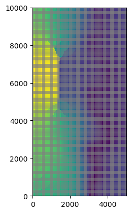
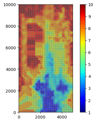
Plot the resampled data
Plot the aquifer top, bottom, and hydraulic conductivity. Also plot the aquifer thickness.
[18]:
mm = flopy.plot.PlotMapView(modelgrid=base_grid)
mm.plot_array(rtop)
mm.plot_grid(lw=0.5, color="0.5");
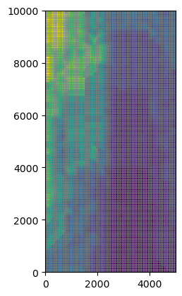
[19]:
mm = flopy.plot.PlotMapView(modelgrid=base_grid)
mm.plot_array(rbot)
mm.plot_grid(lw=0.5, color="0.5");
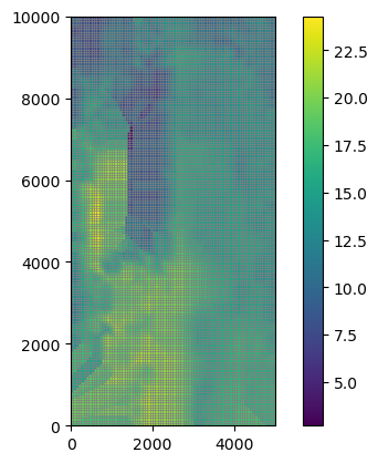
[20]:
mm = flopy.plot.PlotMapView(modelgrid=base_grid)
cb = mm.plot_array(rtop - rbot)
mm.plot_grid(lw=0.5, color="0.5")
plt.colorbar(cb);
[21]:
mm = flopy.plot.PlotMapView(modelgrid=base_grid)
cb = mm.plot_array(rkaq, cmap="jet", vmin=1, vmax=10)
mm.plot_grid(lw=0.5, color="0.5")
plt.colorbar(cb);
Build the model data
Create the bottom of each model layer
Assume that the thickness of each layer at a row, column location is equal.
[22]:
botm = np.zeros(shape3d, dtype=float)
botm[-1, :, :] = rbot[:, :]
layer_thickness = (rtop - rbot) / nlay
for k in reversed(range(nlay - 1)):
    botm[k] = botm[k + 1] + layer_thickness
Create the idomain array
Use the intersection data from the active and inactive shapefiles to create the idomain array
[23]:
idomain = np.zeros((nlay, nrow, ncol), dtype=float)
for i, j in active_cells["cellids"]:
    idomain[:, i, j] = 1
for i, j in bedrock["cellids"]:
    idomain[:, i, j] = 0
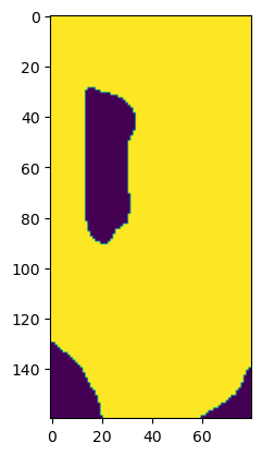
A more pythonic approach
[24]:
idomain_bool = np.zeros((nrow, ncol), dtype=bool)
[25]:
idomain_bool[tuple(zip(*active_cells["cellids"].tolist()))] = True
[26]:
idomain_bool[tuple(zip(*bedrock["cellids"].tolist()))] = False
[27]:
plt.imshow(idomain_bool)
[27]:
<matplotlib.image.AxesImage at 0x14dd33b50>
[28]:
idomain_bool
[28]:
array([[ True,  True,  True, ...,  True,  True,  True],
       [ True,  True,  True, ...,  True,  True,  True],
       [ True,  True,  True, ...,  True,  True,  True],
       ...,
       [False, False, False, ..., False, False, False],
       [False, False, False, ..., False, False, False],
       [False, False, False, ..., False, False, False]])
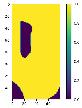
[29]:
idomain = np.zeros((nrow, ncol), dtype=float)
idomain[idomain_bool] = 1
v = plt.imshow(idomain)
plt.colorbar(v)
[29]:
<matplotlib.colorbar.Colorbar at 0x14dae3d90>
[30]:
idomain = np.array([idomain, idomain, idomain])
idomain.shape
[30]:
(3, 160, 80)
Build the well package stress period data
The pumping rates are in the
wellsgeopandas dataframePumping rates are in m\(^3\)/sec
The wells are located in model layer 3
[31]:
wells
[31]:
| FID | Q | geometry | |
|---|---|---|---|
| 0 | 0 | -0.00820 | POINT (3875.000 7875.000) |
| 1 | 1 | -0.00410 | POINT (3125.000 7375.000) |
| 2 | 2 | -0.00390 | POINT (3375.000 5125.000) |
| 3 | 3 | -0.00083 | POINT (2375.000 3625.000) |
| 4 | 4 | -0.00072 | POINT (1375.000 2875.000) |
| 5 | 5 | -0.00430 | POINT (2875.000 1625.000) |
[32]:
well_spd = []
for (i, j), q in zip(well_cells, wells["Q"]):
    well_spd.append([2, i, j, q * 86400.0])
well_spd
[32]:
[[2, 33, 61, -708.48],
 [2, 41, 49, -354.24],
 [2, 77, 53, -336.96],
 [2, 101, 37, -71.712],
 [2, 113, 21, -62.208000000000006],
 [2, 133, 45, -371.52]]
Build the river package stress period data
Calculate the length of the river using the
"lengths"key.The vertical hydraulic conductivity of the river bed sediments is 3.5 m/d.
The thickness of river bottom sediments at the upstream (North) and downstream (South) end of the river is 0.5 and 1.5 meters, respectively.
The river bottom at the upstream and downstream end of the river is 16.5 and 14.5 meters, respectively. The river width at the upstream and downstream end of the river is 5.0 and 10.0 meters, respectively.
The river stage at the upstream and downstream end of the river is 16.6 and 15.5 meters, respectively.
Use the boundname
upstreamfor river cells where the upstream end of the river cell is less than 5000 m from the North end of the model. Use the boundnamedownstreamfor all other river cells.Make sure the river cell is in the upper most layer where the river bottom exceeds the bottom of the cell.
Use the upstream and downstream values to interpolate the river sediment thickness, bottom, width, and stage for each river cell.
The river cells will be connected to model layer 1. The river bottom, width, and stage values should be calculated at the center of the river reach.
[33]:
river_kv = 3.5
river_thickness_up, river_thickness_down = 0.5, 1.5
river_bot_up, river_bot_down = 16.5, 14.5
river_width_up, river_width_down = 5.0, 10.0
stage_up, stage_down = 16.6, 15.5
[34]:
river_length = river_cells["lengths"].sum()
river_length
[34]:
12419.290359618695
[35]:
river_thickness_slope = (
    river_thickness_down - river_thickness_up
) / river_length
[36]:
river_bot_slope = (river_bot_down - river_bot_up) / river_length
[37]:
river_width_slope = (river_width_down - river_width_up) / river_length
[38]:
stage_slope = (stage_down - stage_up) / river_length
[39]:
boundname = "upstream"
total_length = 0.0
river_spd = []
for idx, (cellid, length) in enumerate(
    zip(river_cells["cellids"], river_cells["lengths"])
):
    if total_length >= 5000.0 and boundname == "upstream":
        boundname = "downstream"
    dx = 0.5 * length
    total_length += dx
    river_thickness = river_thickness_up + river_thickness_slope * total_length
    river_bot = river_bot_up + river_bot_slope * total_length
    river_width = river_width_up + river_width_slope * total_length
    river_stage = stage_up + stage_slope * total_length
    conductance = river_kv * length * river_width / river_thickness

    i, j = cellid
    for k in range(nlay):
        if river_bot - river_thickness > botm[k, i, j]:
            riv_layer = k
            break

    river_spd.append(
        [riv_layer, i, j, river_stage, conductance, river_bot, boundname]
    )
    total_length += dx
river_spd[:2], river_spd[-2:]
[39]:
([[0,
   0,
   53,
   16.597225984480367,
   2186.8547136345433,
   16.494956335418845,
   'upstream'],
  [0,
   1,
   53,
   16.591677953441096,
   2176.0166873198878,
   16.484869006256535,
   'upstream']],
 [[0,
   158,
   50,
   15.508347242017402,
   1480.5598623536812,
   14.515176803668005,
   'downstream'],
  [0,
   159,
   50,
   15.502770376374766,
   1460.266817949857,
   14.50503704795412,
   'downstream']])
A more pythonic approach
[40]:
xmid = river_cells["lengths"].cumsum() - 0.5 * river_cells["lengths"]
xp = [0, river_cells["lengths"].cumsum()[-1]]
xp
[40]:
[0, 12419.290359618704]
[41]:
riv_stage = np.interp(xmid, xp, [stage_up, stage_down])
riv_thick = np.interp(xmid, xp, [river_thickness_up, river_thickness_down])
riv_bot = np.interp(xmid, xp, [river_bot_up, river_bot_down])
riv_wid = np.interp(xmid, xp, [river_width_up, river_width_down])
riv_cond = river_kv * river_cells["lengths"] * riv_wid / riv_thick
[42]:
riv_bot_elev = riv_bot - riv_thick
riv_layer = [0 if riv_bot_elev[idx] > botm[0, i, j] else 1 for idx, (i, j) in enumerate(river_cells["cellids"])]
[43]:
riv_bndname = np.full(riv_cond.shape, "upstream", dtype="|S10")
riv_bndname[xmid > 5000.] = "downstream"
[44]:
river_spd = [(riv_layer[idx], i, j, riv_stage[idx], riv_cond[idx], riv_bot[idx], riv_bndname[idx].decode('UTF-8'))
             for idx, (i,j) in enumerate(river_cells["cellids"])]
river_spd[:2], river_spd[-2:]
[44]:
([(0,
   0,
   53,
   16.597225984480367,
   2186.8547136345433,
   16.494956335418845,
   'upstream'),
  (0,
   1,
   53,
   16.591677953441096,
   2176.0166873198878,
   16.484869006256535,
   'upstream')],
 [(0,
   158,
   50,
   15.508347242017402,
   1480.5598623536819,
   14.515176803668004,
   'downstream'),
  (0,
   159,
   50,
   15.502770376374766,
   1460.2668179498573,
   14.50503704795412,
   'downstream')])
Define river observations
[45]:
riv_obs = {
    "riv_obs.csv": [
        ("UPSTREAM", "RIV", "UPSTREAM"),
        ("DOWNSTREAM", "RIV", "DOWNSTREAM"),
    ]
}
Define the constant head cells
Assume the constant head cells are located in all three layers and have values equal to the downstream river stage (stage_down). Make sure the constant head stage is greater that the bottom of the layer.
[46]:
chd_spd = []
for i, j in constant_cells["cellids"]:
    for k in range(nlay):
        if stage_down > botm[k, i, j] and idomain[k, i, j] > 0:
            chd_spd.append((k, i, j, stage_down))
chd_spd[:2], chd_spd[-2:]
[46]:
([(1, 159, 21, 15.5), (2, 159, 21, 15.5)],
 [(1, 159, 59, 15.5), (2, 159, 59, 15.5)])
Define recharge rates
The recharge rate is 0.16000000E-08 m/sec
[47]:
recharge_rate = 0.16000000e-08 * 86400.0
recharge_rate
[47]:
0.00013824
Build the model
Build a steady-state model using the data that you have created. Packages to create:
Simulation
TDIS (1 stress period,
TIME_UNITS='days')IMS (default parameters)
GWF model (
SAVE_FLOWS=True)DIS (
LENGTH_UNITS='meters')IC (
STRT=40.)NPF (Unconfined, same K for all layers,
SAVE_SPECIFIC_DISCHARGE=True,icelltype=1)RCH (array based)
RIV (
BOUNDNAMES=True,addRIVobservations for defined boundnames)CHD
WEL
OC (Save
HEAD ALLandBUDGET ALL)
[48]:
name = "project"
[49]:
sim = flopy.mf6.MFSimulation(sim_name=name, sim_ws=model_ws, exe_name="mf6")
tdis = flopy.mf6.ModflowTdis(sim, time_units="days")
ims = flopy.mf6.ModflowIms(
    sim, outer_maximum=200, inner_maximum=100, linear_acceleration="bicgstab"
)
[50]:
gwf = flopy.mf6.ModflowGwf(
    sim,
    modelname=name,
    save_flows=True,
    newtonoptions="NETWON UNDER_RELAXATION",
)
[51]:
riv_obs
[51]:
{'riv_obs.csv': [('UPSTREAM', 'RIV', 'UPSTREAM'),
  ('DOWNSTREAM', 'RIV', 'DOWNSTREAM')]}
[52]:
dis = flopy.mf6.ModflowGwfdis(
    gwf,
    length_units="meters",
    nlay=nlay,
    nrow=nrow,
    ncol=ncol,
    delr=delr,
    delc=delc,
    top=rtop,
    botm=botm,
    idomain=idomain,
)
ic = flopy.mf6.ModflowGwfic(gwf, strt=40.0)
npf = flopy.mf6.ModflowGwfnpf(
    gwf, save_specific_discharge=True, k=[rkaq, rkaq, rkaq], icelltype=1
)
rch = flopy.mf6.ModflowGwfrcha(gwf, recharge=recharge_rate)
riv = flopy.mf6.ModflowGwfriv(
    gwf, boundnames=True, stress_period_data=river_spd
)
riv.obs.initialize(
    filename=f"{name}.riv.obs",
    digits=9,
    print_input=True,
    continuous=riv_obs,
)
wel = flopy.mf6.ModflowGwfwel(gwf, stress_period_data=well_spd)
chd = flopy.mf6.ModflowGwfchd(gwf, stress_period_data=chd_spd)
oc = flopy.mf6.ModflowGwfoc(
    gwf,
    head_filerecord=f"{name}.hds",
    budget_filerecord=f"{name}.cbc",
    saverecord=[("HEAD", "ALL"), ("BUDGET", "ALL")],
)
Write the model files
[53]:
sim.write_simulation()
writing simulation...
  writing simulation name file...
  writing simulation tdis package...
  writing solution package ims_-1...
  writing model project...
    writing model name file...
    writing package dis...
    writing package ic...
    writing package npf...
    writing package rcha_0...
    writing package riv_0...
INFORMATION: maxbound in ('gwf6', 'riv', 'dimensions') changed to 249 based on size of stress_period_data
    writing package obs_0...
    writing package wel_0...
INFORMATION: maxbound in ('gwf6', 'wel', 'dimensions') changed to 6 based on size of stress_period_data
    writing package chd_0...
INFORMATION: maxbound in ('gwf6', 'chd', 'dimensions') changed to 102 based on size of stress_period_data
    writing package oc...
Run the model
[54]:
sim.run_simulation()
FloPy is using the following executable to run the model: ../../../../../../../.local/share/flopy/bin/mf6
                                   MODFLOW 6
                U.S. GEOLOGICAL SURVEY MODULAR HYDROLOGIC MODEL
                            VERSION 6.4.2 06/28/2023

   MODFLOW 6 compiled Jul 05 2023 20:29:14 with Intel(R) Fortran Intel(R) 64
   Compiler Classic for applications running on Intel(R) 64, Version 2021.7.0
                             Build 20220726_000000

This software has been approved for release by the U.S. Geological
Survey (USGS). Although the software has been subjected to rigorous
review, the USGS reserves the right to update the software as needed
pursuant to further analysis and review. No warranty, expressed or
implied, is made by the USGS or the U.S. Government as to the
functionality of the software and related material nor shall the
fact of release constitute any such warranty. Furthermore, the
software is released on condition that neither the USGS nor the U.S.
Government shall be held liable for any damages resulting from its
authorized or unauthorized use. Also refer to the USGS Water
Resources Software User Rights Notice for complete use, copyright,
and distribution information.


 Run start date and time (yyyy/mm/dd hh:mm:ss): 2024/02/08 12:36:32

 Writing simulation list file: mfsim.lst
 Using Simulation name file: mfsim.nam

    Solving:  Stress period:     1    Time step:     1

 Run end date and time (yyyy/mm/dd hh:mm:ss): 2024/02/08 12:36:33
 Elapsed run time:  0.821 Seconds

 Normal termination of simulation.
[54]:
(True, [])
Post-process the results
Use gwf.output. method to get the observations.
[55]:
myobs = gwf.riv.output.obs().get_data()
myobs.dtype
[55]:
dtype([('totim', '<f8'), ('UPSTREAM', '<f8'), ('DOWNSTREAM', '<f8')])
[56]:
myobs["UPSTREAM"], myobs["DOWNSTREAM"]
[56]:
(array([-1300.79659]), array([-2300.13083]))
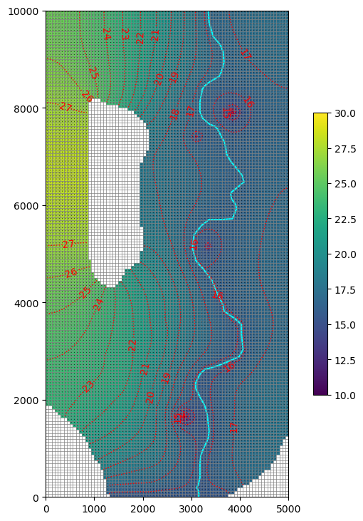
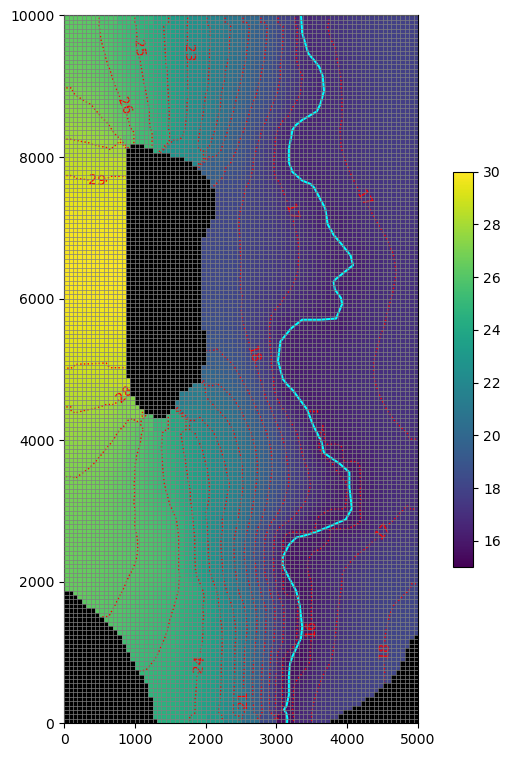
Use gwf.output. method to get the heads and specific discharge. Make a map and cross-sections of the data using flopy.plot methods. Plot specific discharge vectors on the map and cross-sections.
[57]:
head = gwf.output.head().get_data()
fpth = “/Users/jdhughes/Documents/Training/python-for-hydrology/notebooks/part1_flopy/data_project/aquifer_top.asc” np.savetxt(fpth, head[0] + 2.)
[58]:
gwf.output.budget().get_unique_record_names()
[58]:
[b'    FLOW-JA-FACE',
 b'      DATA-SPDIS',
 b'             WEL',
 b'             RIV',
 b'            RCHA',
 b'             CHD']
[59]:
spdis = gwf.output.budget().get_data(text="DATA-SPDIS")[0]
qx, qy, qz = flopy.utils.postprocessing.get_specific_discharge(
    spdis, gwf, head=head
)
[60]:
fig, ax = plt.subplots(
    ncols=1,
    nrows=1,
    figsize=(5, 8),
    constrained_layout=True,
    subplot_kw=dict(aspect="equal"),
)
mm = flopy.plot.PlotMapView(model=gwf, ax=ax, layer=0)
cb = mm.plot_array(head, masked_values=[1e30], vmin=10, vmax=30)
river.plot(color="cyan", ax=mm.ax)
mm.plot_grid(lw=0.5, color="0.5")
mm.plot_vector(qx, qy, normalize=True)
cs = mm.contour_array(
    head,
    masked_values=[1e30],
    colors="red",
    levels=np.arange(10, 28, 1),
    linestyles=":",
    linewidths=1.0,
)
ax.clabel(
    cs,
    inline=True,
    fmt="%1.0f",
    fontsize=10,
    inline_spacing=0.5,
)
# mm.plot_inactive(ibound=idomain)
plt.colorbar(cb, ax=mm.ax, shrink=0.5)

fig.savefig("../figures/freyberg-structured.png", dpi=300);
[61]:
fig, ax = plt.subplots(
    ncols=1,
    nrows=1,
    figsize=(5, 8),
    constrained_layout=True,
    subplot_kw=dict(aspect="equal"),
)

mm = flopy.plot.PlotMapView(model=gwf, ax=ax, layer=0)
cb = mm.plot_array(gwf.dis.top.array, masked_values=[1e30], vmin=15, vmax=30)
river.plot(color="cyan", ax=mm.ax)
mm.plot_grid(lw=0.5, color="0.5", zorder=11)
mm.plot_inactive(zorder=10)
cs = mm.contour_array(
    gwf.dis.top.array,
    colors="red",
    levels=np.arange(15, 31, 1),
    linestyles=":",
    linewidths=1.0,
)
ax.clabel(
    cs,
    inline=True,
    fmt="%1.0f",
    fontsize=10,
    inline_spacing=0.5,
)
plt.colorbar(cb, ax=mm.ax, shrink=0.5)

fig.savefig("../figures/freyberg-structured-grid.png", dpi=300);
[ ]: