03: Loading and visualizing groundwater models
This exercise, we will load an existing model using Flopy, look at some of the inputs, run the model, and load and plot some of the results.
The Pleasant Lake example
The example model is a simplified version of the MODFLOW-6 model published by Fienen and others (2022, 2021), of the area around Pleasant Lake in central Wisconsin, USA. The original report and model files are available at the links below.
Example model details:
Transient MODFLOW-6 simulation with monthly stress periods for calendar year 2012
units of meters and days
4 layers; 100 meter uniform grid spacing
layers 1-3 represent surficial deposits
layer 4 represents Paleozoic bedrock (sandstone)
Transient specified head perimeter boundary (CHD package) from a regional model solution
Transient recharge from a soil water balance model, specified with RCHA
Streams specified with SFR
Pleasant Lake simulated with the Lake Package
Head observations specified with the OBS utility
[1]:
from pathlib import Path
import flopy
import numpy as np
import pandas as pd
import matplotlib.pyplot as plt
[2]:
# make an output folder
output_folder = Path('03-output')
output_folder.mkdir(exist_ok=True)
load a preexisting MODFLOW 6 model
Because this is MODFLOW 6, we need to load the simulation first, and then get the model.
load_only argument to specify the packages that should be loaded.load_only=['dis'][3]:
%%capture
sim_ws = Path('../data/pleasant-lake/')
sim = flopy.mf6.MFSimulation.load('pleasant', sim_ws=str(sim_ws), exe_name='mf6',
                                  #load_only=['dis']
                         )
sim.model_names
[4]:
model = sim.get_model('pleasant')
Visualizing the model
First let’s check that the model grid is correctly located. It is, in this case, because the model has the origin and rotation specified in the DIS package.
[5]:
model.modelgrid
[5]:
xll:552400.0; yll:387200.0; rotation:0.0; units:meters; lenuni:2
[6]:
model.get_package_list()
[6]:
['DIS',
 'IC',
 'NPF',
 'STO',
 'RCHA_0',
 'OC',
 'CHD_OBS',
 'CHD_0',
 'SFR_OBS',
 'SFR_0',
 'LAK_OBS',
 'LAK_LAKTAB',
 'LAK_0',
 'WEL_0',
 'OBS_3']
However, in order to write shapefiles with a .prj file that specifies the coordinate references system (CRS), we need to assign one to the grid (there currently is no CRS input for MODFLOW 6). We can do this by simply specifying an EPSG code to the crs attribute (in this case 3070 for Wisconsin Transverse Mercator).
[7]:
model.modelgrid.crs = 3070
model.modelgrid.units
[7]:
'meters'
Let’s also assign the modelgrid to a variable so we don’t have to type model.modelgrid every time
[8]:
modelgrid = model.modelgrid
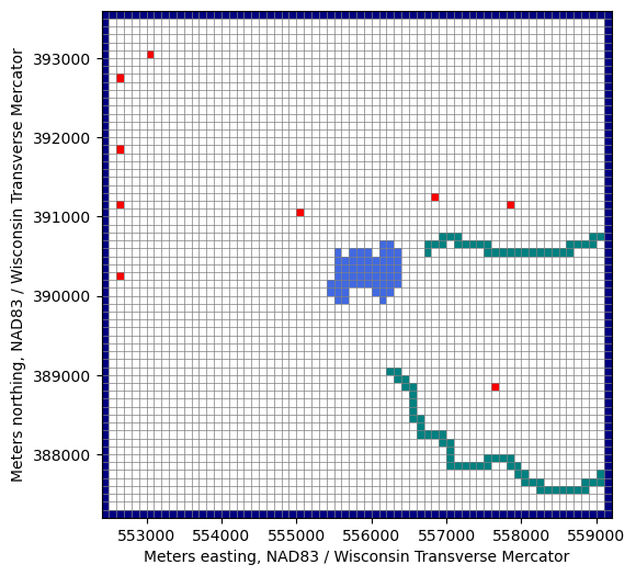
On a map
We can plot the model in the CRS using the PlotMapView object. More examples in the Flopy demo here (for unstructured grids too!): https://github.com/modflowpy/flopy/blob/develop/examples/Notebooks/flopy3.3_PlotMapView.ipynb
[9]:
fig, ax = plt.subplots(figsize=(6, 6))
pmv = flopy.plot.PlotMapView(model, ax=ax)
lc = pmv.plot_grid(lw=0.5)
pmv.plot_bc("WEL", plotAll=True)
pmv.plot_bc("LAK", plotAll=True)
pmv.plot_bc("SFR", plotAll=True)
pmv.plot_bc("CHD", plotAll=True)
ax.set_xlabel(f'{modelgrid.units.capitalize()} easting, {modelgrid.crs.name}')
ax.set_ylabel(f'{modelgrid.units.capitalize()} northing, {modelgrid.crs.name}')
[9]:
Text(0, 0.5, 'Meters northing, NAD83 / Wisconsin Transverse Mercator')
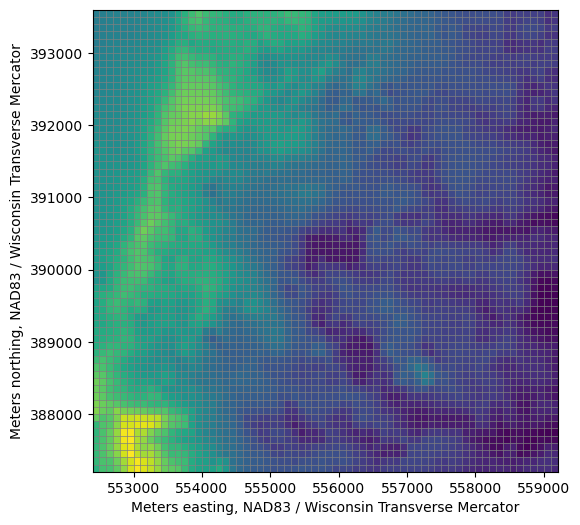
[10]:
fig, ax = plt.subplots(figsize=(6, 6))
pmv = flopy.plot.PlotMapView(model, ax=ax)
lc = pmv.plot_grid(lw=0.5)
top = pmv.plot_array(model.dis.top.array)
ax.set_xlabel(f'{modelgrid.units.capitalize()} easting, {modelgrid.crs.name}')
ax.set_ylabel(f'{modelgrid.units.capitalize()} northing, {modelgrid.crs.name}')
[10]:
Text(0, 0.5, 'Meters northing, NAD83 / Wisconsin Transverse Mercator')
Get the model grid as a GeoPandas GeoDataFrame
[11]:
modelgrid_gdf = modelgrid.geo_dataframe
modelgrid_gdf
[11]:
| geometry | node | row | col | |
|---|---|---|---|---|
| 0 | POLYGON ((552400 393600, 552400 393500, 552500... | 1 | 1 | 1 |
| 1 | POLYGON ((552500 393600, 552500 393500, 552600... | 2 | 1 | 2 |
| 2 | POLYGON ((552600 393600, 552600 393500, 552700... | 3 | 1 | 3 |
| 3 | POLYGON ((552700 393600, 552700 393500, 552800... | 4 | 1 | 4 |
| 4 | POLYGON ((552800 393600, 552800 393500, 552900... | 5 | 1 | 5 |
| ... | ... | ... | ... | ... |
| 4347 | POLYGON ((558700 387300, 558700 387200, 558800... | 4348 | 64 | 64 |
| 4348 | POLYGON ((558800 387300, 558800 387200, 558900... | 4349 | 64 | 65 |
| 4349 | POLYGON ((558900 387300, 558900 387200, 559000... | 4350 | 64 | 66 |
| 4350 | POLYGON ((559000 387300, 559000 387200, 559100... | 4351 | 64 | 67 |
| 4351 | POLYGON ((559100 387300, 559100 387200, 559200... | 4352 | 64 | 68 |
4352 rows × 4 columns
Exporting the model grid to a shapefile
[12]:
modelgrid_gdf.to_file(output_folder / 'pleasant_grid.shp')
Making a cross section through the model
more examples in the Flopy demo here: https://github.com/modflowpy/flopy/blob/develop/examples/Notebooks/flopy3.3_PlotCrossSection.ipynb
By row or column
[13]:
fig, ax = plt.subplots(figsize=(14, 5))
xs = flopy.plot.PlotCrossSection(model=model, line={"row": 30}, ax=ax)
lc = xs.plot_grid()
xs.plot_bc("LAK")
xs.plot_bc("SFR")
ax.set_xlabel(f'Distance, in {modelgrid.units.capitalize()}')
ax.set_ylabel(f'Elevation, in {modelgrid.units.capitalize()}')
[13]:
Text(0, 0.5, 'Elevation, in Meters')

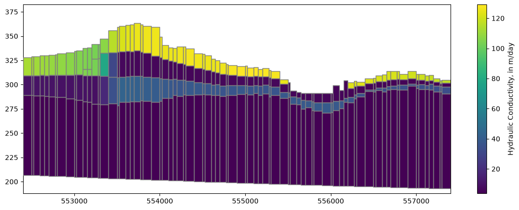
Along an arbitrary line
(and in Geographic Coordinates)
[14]:
fig, ax = plt.subplots(figsize=(14, 5))
xs_line = [(552400, 393000), (552400 + 5000, 393000 - 4000)]
xs = flopy.plot.PlotCrossSection(model=model,
                                 line={"line": xs_line}, ax=ax,
                                 geographic_coords=True)
lc = xs.plot_grid(zorder=4)

pc = xs.plot_array(model.npf.k.array)
fig.colorbar(pc, label='Hydraulic Conductivity, in m/day');
What if we want to look at cross sections for each row or column?
This code allows for every row or column to be visualized in cross section within the Jupyter Notebook session.
[15]:
fig, ax = plt.subplots(figsize=(14, 5))
frames = modelgrid.shape[1] # set frames to number of rows

def update(i):
    ax.cla()
    xs = flopy.plot.PlotCrossSection(model=model, line={"row": i}, ax=ax)
    lc = xs.plot_grid()
    xs.plot_bc("LAK")
    xs.plot_bc("SFR")
    ax.set_title(f"row: {i}")
    ax.set_xlabel(f'Distance, in {modelgrid.units.capitalize()}')
    ax.set_ylabel(f'Elevation, in {modelgrid.units.capitalize()}')
    return

import matplotlib.animation as animation
ani = animation.FuncAnimation(fig=fig, func=update, frames=frames)
plt.close()

from IPython.display import HTML
HTML(ani.to_jshtml())
[15]:
Every input to MODFOW is attached to a Flopy object (with the attribute name of the variable) as a numpy ndarray (for ndarray-type data) or a recarray for tabular or list-type data. For example, we can access the recharge array (4D– nper x nlay x nrow x ncol) with:
model.rcha.recharge.array
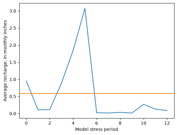
ndarray example: plot spatial average recharge by stress period
To minimize extra typing, it often makes sense to reassign the numpy array to a new variable to work with it further.
[16]:
rch_inches = model.rcha.recharge.array[:, 0, :, :].mean(axis=(1, 2)) * 12 * 30.4 / .3048
fig, ax = plt.subplots()
ax.plot(rch_inches)
ax.axhline(rch_inches.mean(), c='C1')
ax.set_ylabel(f"Average recharge, in monthly inches")
ax.set_xlabel("Model stress period")
[16]:
Text(0.5, 0, 'Model stress period')
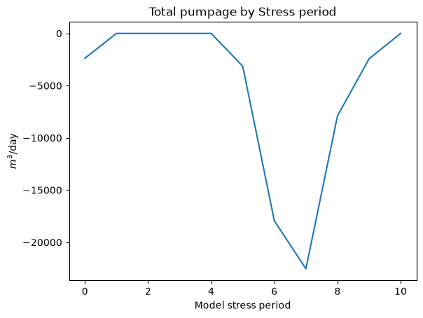
Tabular data example: plot pumping by stress period
Most tabular input for the ‘basic’ stress packages (Constant Head, Drain, General Head, RIV, WEL, etc) are accessible via a stress_period_data attribute.
To access the data, we have to call another
.dataattribute, which gives us a dictionary ofrecarrays by stress period.Any one of these can be converted to a
pandas.DataFrameindividually, or we can make a dataframe of all of them with a simple loop.
[17]:
dfs = []
for kper, df in model.wel.stress_period_data.get_dataframe().items():
    df['per'] = kper
    dfs.append(df)
df = pd.concat(dfs)
df.head()
[17]:
| cellid_layer | cellid_row | cellid_column | q | boundname | per | |
|---|---|---|---|---|---|---|
| 0 | 2 | 24 | 2 | -396.867 | pleasant_2-13-2 | 0 |
| 1 | 2 | 17 | 2 | -409.900 | pleasant_2-9-2 | 0 |
| 2 | 3 | 23 | 44 | 0.000 | pleasant_3-12-23 | 0 |
| 3 | 3 | 25 | 26 | 0.000 | pleasant_3-13-14 | 0 |
| 4 | 3 | 24 | 54 | -878.654 | pleasant_3-13-28 | 0 |
Now we can sum by stress period, or plot individual wells across stress periods
[18]:
df.groupby('per').sum()['q'].plot()
plt.title('Total pumpage by Stress period')
plt.ylabel('$m^3$/day')
plt.xlabel('Model stress period')
[18]:
Text(0.5, 0, 'Model stress period')
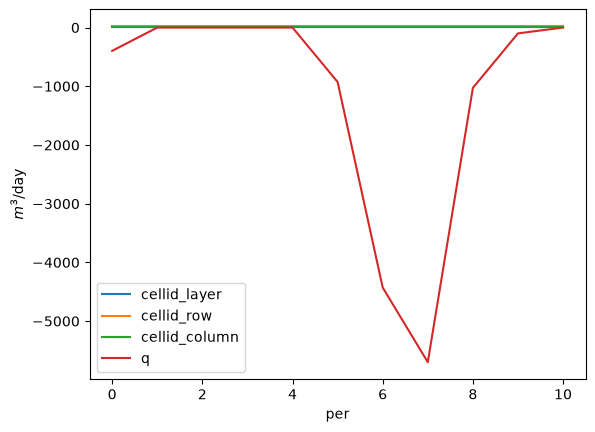
About many gallons did this well pump in stress periods 1 through 12?
[19]:
ax = df.groupby('boundname').get_group('pleasant_2-13-2').plot(x='per')
ax.set_ylabel('$m^3$/day')
[19]:
Text(0, 0.5, '$m^3$/day')
Solution:
get the pumping rates by stress period
[20]:
rates = df.groupby('boundname').get_group('pleasant_2-13-2')[1:]
rates
[20]:
| cellid_layer | cellid_row | cellid_column | q | boundname | per | |
|---|---|---|---|---|---|---|
| 0 | 2 | 24 | 2 | 0.0000 | pleasant_2-13-2 | 1 |
| 0 | 2 | 24 | 2 | 0.0000 | pleasant_2-13-2 | 4 |
| 0 | 2 | 24 | 2 | -926.7360 | pleasant_2-13-2 | 5 |
| 0 | 2 | 24 | 2 | -4428.3600 | pleasant_2-13-2 | 6 |
| 0 | 2 | 24 | 2 | -5699.1800 | pleasant_2-13-2 | 7 |
| 0 | 2 | 24 | 2 | -1027.5000 | pleasant_2-13-2 | 8 |
| 0 | 2 | 24 | 2 | -99.1399 | pleasant_2-13-2 | 9 |
| 0 | 2 | 24 | 2 | 0.0000 | pleasant_2-13-2 | 10 |
Google “python get days in month” or similar (simply using 30.4 would be fine too for an approximate answer)
[21]:
import calendar
rates['days'] = [calendar.monthrange(2012,m)[1] for m in rates['per']]
multiply the days by the daily pumping rate to get the totals; convert units and sum
[22]:
rates
[22]:
| cellid_layer | cellid_row | cellid_column | q | boundname | per | days | |
|---|---|---|---|---|---|---|---|
| 0 | 2 | 24 | 2 | 0.0000 | pleasant_2-13-2 | 1 | 31 |
| 0 | 2 | 24 | 2 | 0.0000 | pleasant_2-13-2 | 4 | 30 |
| 0 | 2 | 24 | 2 | -926.7360 | pleasant_2-13-2 | 5 | 31 |
| 0 | 2 | 24 | 2 | -4428.3600 | pleasant_2-13-2 | 6 | 30 |
| 0 | 2 | 24 | 2 | -5699.1800 | pleasant_2-13-2 | 7 | 31 |
| 0 | 2 | 24 | 2 | -1027.5000 | pleasant_2-13-2 | 8 | 31 |
| 0 | 2 | 24 | 2 | -99.1399 | pleasant_2-13-2 | 9 | 30 |
| 0 | 2 | 24 | 2 | 0.0000 | pleasant_2-13-2 | 10 | 31 |
[23]:
rates['gallons'] = rates['q'] * rates['days'] * 264.172
print(f"{rates['gallons'].sum():,}")
-98,557,525.66559602
[24]:
sim.run_simulation()
FloPy is using the following executable to run the model: ../../../../../../../../../.local/bin/mf6
                                   MODFLOW 6
                U.S. GEOLOGICAL SURVEY MODULAR HYDROLOGIC MODEL
                            VERSION 6.7.0 02/05/2026

   MODFLOW 6 compiled Feb 05 2026 22:38:38 with Intel(R) Fortran Intel(R) 64
   Compiler Classic for applications running on Intel(R) 64, Version 2021.6.0
                             Build 20220226_000000

This software has been approved for release by the U.S. Geological
Survey (USGS). Although the software has been subjected to rigorous
review, the USGS reserves the right to update the software as needed
pursuant to further analysis and review. No warranty, expressed or
implied, is made by the USGS or the U.S. Government as to the
functionality of the software and related material nor shall the
fact of release constitute any such warranty. Furthermore, the
software is released on condition that neither the USGS nor the U.S.
Government shall be held liable for any damages resulting from its
authorized or unauthorized use. Also refer to the USGS Water
Resources Software User Rights Notice for complete use, copyright,
and distribution information.


 MODFLOW runs in SEQUENTIAL mode

 Run start date and time (yyyy/mm/dd hh:mm:ss): 2026/07/16  2:10:20

 Writing simulation list file: mfsim.lst
 Using Simulation name file: mfsim.nam

    Solving:  Stress period:     1    Time step:     1
    Solving:  Stress period:     2    Time step:     1
    Solving:  Stress period:     3    Time step:     1
    Solving:  Stress period:     4    Time step:     1
    Solving:  Stress period:     5    Time step:     1
    Solving:  Stress period:     6    Time step:     1
    Solving:  Stress period:     7    Time step:     1
    Solving:  Stress period:     8    Time step:     1
    Solving:  Stress period:     9    Time step:     1
    Solving:  Stress period:    10    Time step:     1
    Solving:  Stress period:    11    Time step:     1
    Solving:  Stress period:    12    Time step:     1
    Solving:  Stress period:    13    Time step:     1

 Run end date and time (yyyy/mm/dd hh:mm:ss): 2026/07/16  2:10:22
 Elapsed run time:  1.954 Seconds


WARNING REPORT:

  1. OPTIONS BLOCK VARIABLE 'UNIT_CONVERSION' IN FILE 'pleasant.sfr' WAS
     DEPRECATED IN VERSION 6.4.2. SETTING UNIT_CONVERSION DIRECTLY.
 Normal termination of simulation.
[24]:
(True, [])
Getting MODFLOW output from the model object
With MODFLOW 6 models, we can get the output from the model object, without having to reference the output files.
In Flopy, MODFLOW binary output is read using objects that represent the various file types.
[25]:
headfile_object = model.output.head()
headfile_object
[25]:
<flopy.utils.binaryfile.HeadFile at 0x7f2b20934440>
The output file objects include various methods and attributes with information about the output. For example, the elapsed simulation times with output recrods.
[26]:
headfile_object.get_times()
[26]:
[np.float64(1.0),
 np.float64(32.0),
 np.float64(61.0),
 np.float64(92.0),
 np.float64(122.0),
 np.float64(153.0),
 np.float64(183.0),
 np.float64(214.0),
 np.float64(245.0),
 np.float64(275.0),
 np.float64(306.0),
 np.float64(336.0),
 np.float64(367.0)]
Including a get_data() method to get the output values:
[27]:
heads = headfile_object.get_data(kstpkper=(0, 0))
[28]:
sfr_output_object = model.sfr.output
sfr_output_object
[28]:
MF6Output Class for sfr_0
Available output methods include:
.zonebudget()
.budget()
.budgetcsv()
.package_convergence()
.obs()
.stage()
[29]:
sfr_stage = sfr_output_object.stage().get_data()[0, 0, :]
Cell Budget output works the same way.
In this case, we specified save_flows as an option in the various packages to save flux output for those packages, include fluxes to and from the Lake and SFR Packages.
[30]:
cbc_file_object = model.output.budget()
cbc_file_object.get_unique_record_names()
[30]:
[np.bytes_(b'          STO-SS'),
 np.bytes_(b'          STO-SY'),
 np.bytes_(b'    FLOW-JA-FACE'),
 np.bytes_(b'             WEL'),
 np.bytes_(b'            RCHA'),
 np.bytes_(b'             CHD'),
 np.bytes_(b'             SFR'),
 np.bytes_(b'             LAK')]
Cell Budget results are returned in a list that allows for auxilliary information besides the output to be included in subsequent items.
The values are the first item.
[31]:
lake_fluxes = cbc_file_object.get_data(text='lak', full3D=True)[0]
Especially for structured (layer, row, column) grids, we usually want to specify full3D=True. This returns the results in a 3D Numpy array.
Otherwise, results are returned in a Numpy recarray, referenced by unique node numbers.
[32]:
cbc_file_object.get_data(text='lak')[0][:5]
[32]:
rec.array([(6560, 1, -163.5854572 ), (6566, 1,   85.47697217),
           (6763, 1, -201.692521  ), (6633, 1,   53.84431952),
           (6563, 1,   -8.88752784)],
          dtype=[('node', '<i4'), ('node2', '<i4'), ('q', '<f8')])
[33]:
cbc_file_object = model.output.budget()
lake_fluxes = cbc_file_object.get_data(text='lak', full3D=True)[0].sum(axis=0)
sfr_fluxes = cbc_file_object.get_data(text='sfr', full3D=True)[0]
Alternatively, read MODFLOW binary output from the files
[34]:
from flopy.utils import binaryfile as bf

headfile_object = bf.HeadFile(sim_ws / f"{model.name}.hds")
heads_from_the_file = headfile_object.get_data(kstpkper=(0, 0))
[35]:
cbc_file_object = bf.CellBudgetFile(sim_ws / f"{model.name}.cbc")
cbc_fluxes_from_the_file = cbc_file_object.get_data(kstpkper=(0, 0), full3D=True)[0]
MODFLOW 6 CSV observation output can also be easily read using pandas
[36]:
lak_output = pd.read_csv(sim_ws / 'lake1.obs.csv')
lak_output.head()
[36]:
| time | STAGE | INFLOW | RAINFALL | RUNOFF | LAK | WITHDRAWAL | EVAPORATION | STORAGE | VOLUME | SURFACE-AREA | WETTED-AREA | CONDUCTANCE | |
|---|---|---|---|---|---|---|---|---|---|---|---|---|---|
| 0 | 1.0 | 302.000818 | 0.0 | 2048.465617 | 0.0 | 1432.796191 | 0.0 | -480.872306 | 0.000000 | 4820408.264 | 763500.0 | 540000.0 | 13694.60149 |
| 1 | 32.0 | 301.950066 | 0.0 | 494.206161 | 0.0 | 1499.121637 | 0.0 | -196.705306 | 1249.989555 | 4781658.588 | 763500.0 | 540000.0 | 13694.60149 |
| 2 | 61.0 | 301.903708 | 0.0 | 668.720690 | 0.0 | 1511.548756 | 0.0 | -311.952356 | 1220.489893 | 4746264.381 | 763500.0 | 540000.0 | 13694.60149 |
| 3 | 92.0 | 301.884950 | 0.0 | 1851.709161 | 0.0 | 1368.143521 | 0.0 | -873.164663 | 461.989594 | 4731942.704 | 763500.0 | 540000.0 | 13694.60149 |
| 4 | 122.0 | 301.889281 | 0.0 | 2333.612300 | 0.0 | 1096.265713 | 0.0 | -1055.726856 | -110.223034 | 4735249.395 | 763500.0 | 540000.0 | 13694.60149 |
[37]:
head_obs_output = pd.read_csv(sim_ws / f"{model.name}.head.obs")
head_obs_output.head()
[37]:
| time | 00400037_UWSP | 00400037_UWSP.1 | 00400037_UWSP.2 | 00400037_UWSP.3 | 00400041_UWSP | 00400041_UWSP.1 | 00400041_UWSP.2 | 00400041_UWSP.3 | 10019264_LK | ... | YH229.2 | YH229.3 | YQ987 | YQ987.1 | YQ987.2 | YQ987.3 | YS864 | YS864.1 | YS864.2 | YS864.3 | |
|---|---|---|---|---|---|---|---|---|---|---|---|---|---|---|---|---|---|---|---|---|---|
| 0 | 1.0 | 310.161509 | 310.152440 | 310.146632 | 309.972583 | 294.571188 | 294.533753 | 294.507520 | 294.460828 | 287.057064 | ... | 301.671867 | 301.833545 | 302.314533 | 302.324774 | 302.335628 | 302.712518 | 312.448733 | 312.427510 | 312.400785 | 312.395162 |
| 1 | 32.0 | 310.114717 | 310.114717 | 310.108406 | 309.932164 | 294.496467 | 294.460880 | 294.436082 | 294.403306 | 287.002266 | ... | 301.609129 | 301.772555 | 302.230838 | 302.244670 | 302.258673 | 302.652591 | 312.387007 | 312.383407 | 312.353905 | 312.348160 |
| 2 | 61.0 | 310.078745 | 310.078745 | 310.072239 | 309.894409 | 294.432037 | 294.396652 | 294.372019 | 294.340104 | 286.969376 | ... | 301.559509 | 301.721138 | 302.179090 | 302.193726 | 302.208416 | 302.605806 | 312.345221 | 312.339465 | 312.307319 | 312.299521 |
| 3 | 92.0 | 310.051664 | 310.051664 | 310.048010 | 309.878756 | 294.459305 | 294.424027 | 294.399453 | 294.367593 | 287.008239 | ... | 301.576502 | 301.736277 | 302.211276 | 302.221966 | 302.233239 | 302.614153 | 312.367330 | 312.340335 | 312.309477 | 312.304597 |
| 4 | 122.0 | 310.100468 | 310.085611 | 310.082751 | 309.915603 | 294.568056 | 294.532587 | 294.507949 | 294.476668 | 287.084117 | ... | 301.647729 | 301.809016 | 302.261779 | 302.269823 | 302.278917 | 302.655915 | 312.416061 | 312.379106 | 312.355470 | 312.358140 |
5 rows × 550 columns
The head solution is reported for each layer.
We can use the
get_water_tableutility to get a 2D surface of the water table position in each cell.To accurately portray the water table around the lake, we can read the lake stage from the observation file and assign it to the relevant cells in the water table array.
Otherwise, depending on how the lake is constructed, the lake area would be shown as a nodata/no-flow area, or as the heads in the groundwater system below the lakebed.
In this case, we are getting the solution from the initial steady-state period
[38]:
from flopy.utils.postprocessing import get_water_table

water_table = get_water_table(heads)

# add the lake stage to the water table
stage = lak_output['STAGE'][0]
cnd = pd.DataFrame(model.lak.connectiondata.array)
k, i, j = zip(*cnd['cellid'])
water_table[i, j] = stage
# add the SFR stage as well
# get the SFR cell i, j locations
# by unpacking the cellid tuples in the packagedata
sfr_k, sfr_i, sfr_j = zip(*model.sfr.packagedata.array['cellid'])
water_table[sfr_i, sfr_j] = sfr_stage
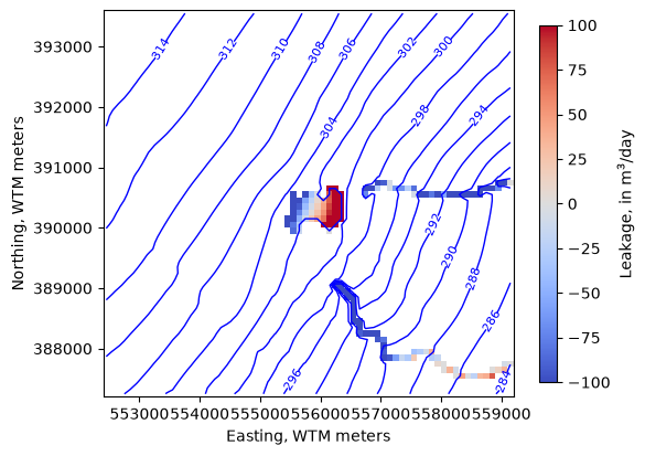
We can add output to a PlotMapView instance as arrays
[39]:
levels=np.arange(280, 315, 2)

fig, ax = plt.subplots(figsize=(6, 6))
pmv = flopy.plot.PlotMapView(model, ax=ax)
ctr = pmv.contour_array(water_table, levels=levels,
                        linewidths=1, colors='b')
labels = pmv.ax.clabel(ctr, inline=True, fontsize=8, inline_spacing=1)
vmin, vmax = -100, 100
im = pmv.plot_array(lake_fluxes, cmap='coolwarm', vmin=vmin, vmax=vmax)
im = pmv.plot_array(sfr_fluxes.sum(axis=0), cmap='coolwarm', vmin=vmin, vmax=vmax)
cb = fig.colorbar(im, shrink=0.7, label='Leakage, in m$^3$/day')
ax.set_ylabel("Northing, WTM meters")
ax.set_xlabel("Easting, WTM meters")
ax.set_aspect(1)
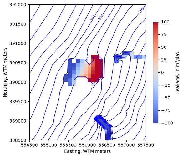
Zoom in on the lake
[40]:
levels=np.arange(280, 315, 1)
new_extent = (554500, 557500, 388500, 392000)

fig, ax = plt.subplots(figsize=(6, 6))
pmv = flopy.plot.PlotMapView(model, ax=ax, extent=new_extent)
ctr = pmv.contour_array(water_table, levels=levels,
                        linewidths=1, colors='b')
labels = pmv.ax.clabel(ctr, inline=True, fontsize=8, inline_spacing=1)
vmin, vmax = -100, 100
im = pmv.plot_array(lake_fluxes, cmap='coolwarm', vmin=vmin, vmax=vmax)
im = pmv.plot_array(sfr_fluxes.sum(axis=0), cmap='coolwarm', vmin=vmin, vmax=vmax)
cb = fig.colorbar(im, shrink=0.7, label='Leakage, in m$^3$/day')
ax.set_ylabel("Northing, WTM meters")
ax.set_xlabel("Easting, WTM meters")
ax.set_aspect(1)
We can use the export_array utility to make a GeoTIFF of any 2D array on a structured grid. For example, make a raster of the simulated water table.
[41]:
from flopy.export.utils import export_array

export_array(model.modelgrid, str(output_folder / 'water_table.tif'), water_table)
/home/runner/micromamba/envs/pyclass-docs/lib/python3.14/site-packages/pyproj/crs/crs.py:1295: UserWarning: You will likely lose important projection information when converting to a PROJ string from another format. See: https://proj.org/faq.html#what-is-the-best-format-for-describing-coordinate-reference-systems
  proj = self._crs.to_proj4(version=version)
A common issue with groundwater flow models is overpressurization- where heads above the land surface are simulated. Sometimes, these indicate natural wetlands that aren’t explicitly simulated in the model, but other times they are a sign of unrealistic parameters. Use the information in this lesson to answer the following questions:
Does this model solution have any overpressiuzation? If so, where? Is it appropriate?
What is the maximum value of overpressurization?
What is the maximum depth to water simulated? Where are the greatest depths to water? Do they look appropriate?
Solution
Make a numpy array of overpressurization and get the max and min values
[42]:
op = water_table - model.dis.top.array
op.max(), op.min()
[42]:
(np.float64(11.120818299999996), np.float64(-76.35338698486248))
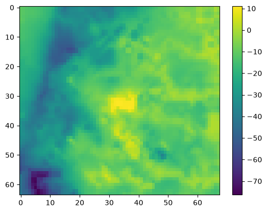
Plot it
[43]:
plt.imshow(op); plt.colorbar()
[43]:
<matplotlib.colorbar.Colorbar at 0x7f2b163f9550>
Export a raster of overpressurization so we can compare it against air photos (or mapped wetlands if we have them!)
[44]:
export_array(model.modelgrid, str(output_folder / 'op.tif'), op)
The highest levels of overpressurization correspond to Pleasant Lake, where the model top represents the lake bottom. Other areas of OP appear to correspond to lakes or wetlands, especially the spring complex south of Pleasant Lake, where Tagatz Creek originates.
The greatest depths to water correspond to a topographic high in the southwest part of the model domain. A cross section through the area confirms that it is a bedrock high that rises more than 50 meters above the surrounding topography, so a depth to water of 76 meters in this area seems reasonable.
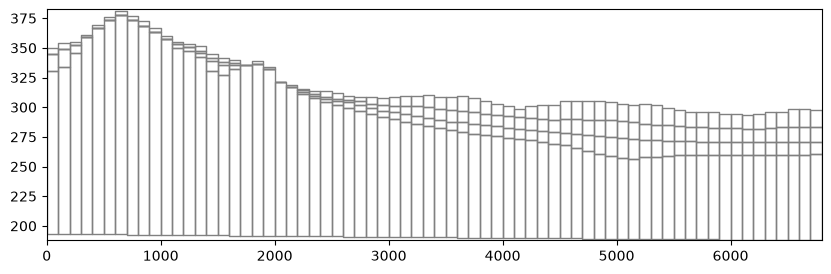
[45]:
fig, ax = plt.subplots(figsize=(10, 3))
xs = flopy.plot.PlotCrossSection(model=model, line={"row": 62}, ax=ax)
lc = xs.plot_grid()
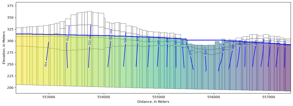
We can also view output in cross section. In this case, PlotMatView plots the head solution where the model is saturated. We can add the water table we created above that includes the lake surface.
[46]:
fig, ax = plt.subplots(figsize=(15, 5))
xs_line = [(552400, 393000), (552400 + 5000, 393000 - 4000)]
xs = flopy.plot.PlotCrossSection(model=model,
                                 line={"line": xs_line},
                                 #line={"row": 32},
                                 ax=ax,
                                 geographic_coords=True)
lc = xs.plot_grid()
pc = xs.plot_array(heads, head=heads, alpha=0.5, masked_values=[1e30])
ctr = xs.contour_array(heads, head=heads, levels=levels, colors="b", masked_values=[1e30])
surf = xs.plot_surface(water_table, masked_values=[1e30], color="blue", lw=2)

labels = pmv.ax.clabel(
    ctr, inline=True,
    fontsize=8, inline_spacing=5)

ax.set_xlabel(f'Distance, in {modelgrid.units.capitalize()}')
ax.set_ylabel(f'Elevation, in {modelgrid.units.capitalize()}')
[46]:
Text(0, 0.5, 'Elevation, in Meters')
In this model, head “observations” were specified at various locations using the MODFLOW 6 Observation Utility. MODFLOW reports simulated values of head at these locations, which can then be compared with equivalent field observations for model parameter estimation.
Earlier we obtained a DataFrame of Lake Package observation output for pleasant lake by reading in ‘lake1.obs.csv’ with pandas. We can read the head observation output with pandas too.
[47]:
headobs = pd.read_csv(sim_ws / 'pleasant.head.obs')
headobs.head()
[47]:
| time | 00400037_UWSP | 00400037_UWSP.1 | 00400037_UWSP.2 | 00400037_UWSP.3 | 00400041_UWSP | 00400041_UWSP.1 | 00400041_UWSP.2 | 00400041_UWSP.3 | 10019264_LK | ... | YH229.2 | YH229.3 | YQ987 | YQ987.1 | YQ987.2 | YQ987.3 | YS864 | YS864.1 | YS864.2 | YS864.3 | |
|---|---|---|---|---|---|---|---|---|---|---|---|---|---|---|---|---|---|---|---|---|---|
| 0 | 1.0 | 310.161509 | 310.152440 | 310.146632 | 309.972583 | 294.571188 | 294.533753 | 294.507520 | 294.460828 | 287.057064 | ... | 301.671867 | 301.833545 | 302.314533 | 302.324774 | 302.335628 | 302.712518 | 312.448733 | 312.427510 | 312.400785 | 312.395162 |
| 1 | 32.0 | 310.114717 | 310.114717 | 310.108406 | 309.932164 | 294.496467 | 294.460880 | 294.436082 | 294.403306 | 287.002266 | ... | 301.609129 | 301.772555 | 302.230838 | 302.244670 | 302.258673 | 302.652591 | 312.387007 | 312.383407 | 312.353905 | 312.348160 |
| 2 | 61.0 | 310.078745 | 310.078745 | 310.072239 | 309.894409 | 294.432037 | 294.396652 | 294.372019 | 294.340104 | 286.969376 | ... | 301.559509 | 301.721138 | 302.179090 | 302.193726 | 302.208416 | 302.605806 | 312.345221 | 312.339465 | 312.307319 | 312.299521 |
| 3 | 92.0 | 310.051664 | 310.051664 | 310.048010 | 309.878756 | 294.459305 | 294.424027 | 294.399453 | 294.367593 | 287.008239 | ... | 301.576502 | 301.736277 | 302.211276 | 302.221966 | 302.233239 | 302.614153 | 312.367330 | 312.340335 | 312.309477 | 312.304597 |
| 4 | 122.0 | 310.100468 | 310.085611 | 310.082751 | 309.915603 | 294.568056 | 294.532587 | 294.507949 | 294.476668 | 287.084117 | ... | 301.647729 | 301.809016 | 302.261779 | 302.269823 | 302.278917 | 302.655915 | 312.416061 | 312.379106 | 312.355470 | 312.358140 |
5 rows × 550 columns
Head observations can also be accessed via the .output attribute for their respective package. First we have to find the name associated with that package though. We can get this by calling get_package_list(). Looks like "OBS_3" is it (since the only OBS packages in the model is for heads).
[48]:
model.get_package_list()
[48]:
['DIS',
 'IC',
 'NPF',
 'STO',
 'RCHA_0',
 'OC',
 'CHD_OBS',
 'CHD_0',
 'SFR_OBS',
 'SFR_0',
 'LAK_OBS',
 'LAK_LAKTAB',
 'LAK_0',
 'WEL_0',
 'OBS_3']
Next let’s query the available output methods:
[49]:
model.obs_3.output.methods()
[49]:
['obs()']
Now get the output. It comes back as a Numpy recarray be default, but we can easily cast it to a DataFrame.
[50]:
pd.DataFrame(model.obs_3.output.obs().get_data())
[50]:
| totim | 00400037_UWSP | 00400037_UWSP_1 | 00400037_UWSP_2 | 00400037_UWSP_3 | 00400041_UWSP | 00400041_UWSP_1 | 00400041_UWSP_2 | 00400041_UWSP_3 | 10019264_LK | ... | YH229_2 | YH229_3 | YQ987 | YQ987_1 | YQ987_2 | YQ987_3 | YS864 | YS864_1 | YS864_2 | YS864_3 | |
|---|---|---|---|---|---|---|---|---|---|---|---|---|---|---|---|---|---|---|---|---|---|
| 0 | 1.0 | 310.161509 | 310.152440 | 310.146632 | 309.972583 | 294.571188 | 294.533753 | 294.507520 | 294.460828 | 287.057064 | ... | 301.671867 | 301.833545 | 302.314533 | 302.324774 | 302.335628 | 302.712518 | 312.448733 | 312.427510 | 312.400785 | 312.395162 |
| 1 | 32.0 | 310.114717 | 310.114717 | 310.108406 | 309.932164 | 294.496467 | 294.460880 | 294.436082 | 294.403306 | 287.002266 | ... | 301.609129 | 301.772555 | 302.230838 | 302.244670 | 302.258673 | 302.652591 | 312.387007 | 312.383407 | 312.353905 | 312.348160 |
| 2 | 61.0 | 310.078745 | 310.078745 | 310.072239 | 309.894409 | 294.432037 | 294.396652 | 294.372019 | 294.340104 | 286.969376 | ... | 301.559509 | 301.721138 | 302.179090 | 302.193726 | 302.208416 | 302.605806 | 312.345221 | 312.339465 | 312.307319 | 312.299521 |
| 3 | 92.0 | 310.051664 | 310.051664 | 310.048010 | 309.878756 | 294.459305 | 294.424027 | 294.399453 | 294.367593 | 287.008239 | ... | 301.576502 | 301.736277 | 302.211276 | 302.221966 | 302.233239 | 302.614153 | 312.367330 | 312.340335 | 312.309477 | 312.304597 |
| 4 | 122.0 | 310.100468 | 310.085611 | 310.082751 | 309.915603 | 294.568056 | 294.532587 | 294.507949 | 294.476668 | 287.084117 | ... | 301.647729 | 301.809016 | 302.261779 | 302.269823 | 302.278917 | 302.655915 | 312.416061 | 312.379106 | 312.355470 | 312.358140 |
| 5 | 153.0 | 310.235321 | 310.199075 | 310.194833 | 310.027845 | 294.796498 | 294.758553 | 294.732077 | 294.686100 | 287.220264 | ... | 301.813281 | 301.975636 | 302.396360 | 302.398604 | 302.402832 | 302.767035 | 312.575743 | 312.507196 | 312.491556 | 312.497321 |
| 6 | 183.0 | 310.163825 | 310.163825 | 310.157828 | 309.981661 | 294.621679 | 294.576452 | 294.544147 | 294.442276 | 287.107788 | ... | 301.718030 | 301.875807 | 302.246336 | 302.255837 | 302.266475 | 302.665988 | 312.425419 | 312.425419 | 312.381849 | 312.318708 |
| 7 | 214.0 | 310.119995 | 310.119995 | 310.112096 | 309.925188 | 294.454998 | 294.409225 | 294.376607 | 294.278295 | 287.028352 | ... | 301.628453 | 301.781572 | 302.117821 | 302.127804 | 302.139043 | 302.556083 | 312.285063 | 312.285063 | 312.219997 | 312.100432 |
| 8 | 245.0 | 310.070133 | 310.070133 | 310.060672 | 309.866641 | 294.339769 | 294.298032 | 294.268599 | 294.199605 | 286.964157 | ... | 301.548295 | 301.700672 | 302.035369 | 302.047486 | 302.060517 | 302.485163 | 312.145582 | 312.145582 | 312.082348 | 311.981909 |
| 9 | 275.0 | 310.017054 | 310.017054 | 310.006291 | 309.806911 | 294.265782 | 294.228015 | 294.201671 | 294.159662 | 286.918126 | ... | 301.480559 | 301.633655 | 301.967317 | 301.980463 | 301.994352 | 302.422722 | 312.023952 | 312.023952 | 311.967218 | 311.886852 |
| 10 | 306.0 | 309.959204 | 309.959204 | 309.947646 | 309.746573 | 294.238342 | 294.205638 | 294.183002 | 294.157879 | 286.889451 | ... | 301.423747 | 301.579611 | 302.097603 | 302.099598 | 302.103294 | 302.453426 | 311.936403 | 311.936403 | 311.895809 | 311.855302 |
| 11 | 336.0 | 309.901502 | 309.901502 | 309.889458 | 309.687545 | 294.192535 | 294.159201 | 294.136085 | 294.109999 | 286.868051 | ... | 301.378561 | 301.534836 | 301.999046 | 302.008866 | 302.019466 | 302.404509 | 311.866721 | 311.866721 | 311.832468 | 311.803879 |
| 12 | 367.0 | 309.841147 | 309.841147 | 309.828881 | 309.627000 | 294.137787 | 294.104305 | 294.081079 | 294.055085 | 286.846760 | ... | 301.335208 | 301.489307 | 301.935854 | 301.949670 | 301.963715 | 302.363014 | 311.801949 | 311.801949 | 311.770597 | 311.747920 |
13 rows × 550 columns
In MODFLOW 6, we can use boundnames to create observations for groups of cells. For example, in this model, each head value specified in the Constant Head (CHD) Package has a boundname of east, west, north or south, to indicate the side of the model perimeter it’s on.
Example of boundnames specified in an external input file for the CHD Package:
[51]:
pd.read_csv(sim_ws / 'external/chd_001.dat', sep=r'\s+')
[51]:
| #k | i | j | head | boundname | |
|---|---|---|---|---|---|
| 0 | 1 | 1 | 68 | 297.761 | east |
| 1 | 1 | 2 | 68 | 297.475 | east |
| 2 | 1 | 3 | 68 | 297.155 | east |
| 3 | 1 | 4 | 68 | 296.871 | east |
| 4 | 1 | 5 | 68 | 296.628 | east |
| ... | ... | ... | ... | ... | ... |
| 763 | 4 | 1 | 63 | 299.500 | north |
| 764 | 4 | 1 | 64 | 299.160 | north |
| 765 | 4 | 1 | 65 | 298.815 | north |
| 766 | 4 | 1 | 66 | 298.469 | north |
| 767 | 4 | 1 | 67 | 298.117 | north |
768 rows × 5 columns
The Constant Head Observation Utility input is then set up like so:
BEGIN options
END options

BEGIN continuous  FILEOUT  pleasant.chd.obs.output.csv
# obsname obstype ID
  east  chd  east
  west  chd  west
  north  chd  north
  south  chd  south
END continuous  FILEOUT  pleasant.chd.obs.output.csv
The resulting observation output (net flow across the boundary faces in model units of cubic meters per day) can be found in pleasant.chd.obs.output.csv:
[52]:
df = pd.read_csv(sim_ws / 'pleasant.chd.obs.output.csv')
df.index = df['time']
df.head()
[52]:
| time | EAST | WEST | NORTH | SOUTH | |
|---|---|---|---|---|---|
| time | |||||
| 1.0 | 1.0 | -34777.174522 | 6212.364587 | 17421.976405 | -9693.413528 |
| 32.0 | 32.0 | -34508.241785 | 6363.316750 | 17572.839997 | -9487.079655 |
| 61.0 | 61.0 | -34204.575965 | 6300.560999 | 17485.626670 | -9557.938536 |
| 92.0 | 92.0 | -34234.776102 | 5908.645868 | 17351.380660 | -9853.130777 |
| 122.0 | 122.0 | -34721.889343 | 5359.082084 | 17203.878073 | -10100.990774 |
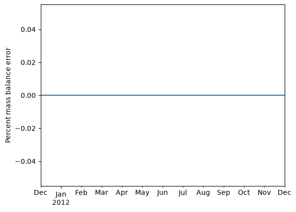
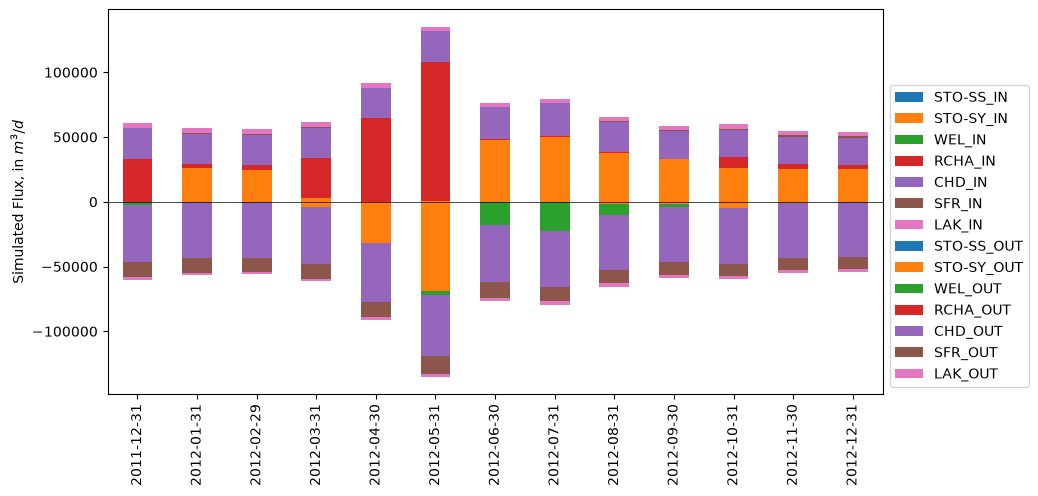
The Mf6ListBudget and MfListBudget (for earlier MODFLOW versions) utilities can assemble the global mass balance output (printed in the Listing file) into a DataFrame. A start_datetime can be added to convert the MODFLOW time to actual dates.
Note: The start_datetime functionality is unaware of steady-state periods, so if we put in the actual model start date of 2012-01-01, the 1-day initial steady-state will be included, resulting in the stress periods being offset by one day. Also note that the dates here represent the end of each stress period.
[53]:
from flopy.utils import Mf6ListBudget
[54]:
mfl = Mf6ListBudget(sim_ws / 'pleasant.list')
flux, vol = mfl.get_dataframes(start_datetime='2011-12-30')
flux.head()
[54]:
| STO-SS_IN | STO-SY_IN | WEL_IN | RCHA_IN | CHD_IN | SFR_IN | LAK_IN | TOTAL_IN | STO-SS_OUT | STO-SY_OUT | WEL_OUT | RCHA_OUT | CHD_OUT | SFR_OUT | LAK_OUT | TOTAL_OUT | IN-OUT | PERCENT_DISCREPANCY | |
|---|---|---|---|---|---|---|---|---|---|---|---|---|---|---|---|---|---|---|
| 2011-12-31 | 0.0000 | 0.000000 | 0.0 | 33188.867188 | 23435.904297 | 349.638306 | 3680.284180 | 60654.695312 | 0.000000 | 0.000000 | 2383.022705 | 0.0 | 44272.152344 | 11781.069336 | 2217.934814 | 60654.175781 | 0.517400 | 0.0 |
| 2012-01-31 | 6.7081 | 25877.734375 | 0.0 | 3485.810791 | 23184.136719 | 518.563782 | 3719.994385 | 56792.949219 | 0.241800 | 156.215195 | 0.000000 | 0.0 | 43243.300781 | 11221.008789 | 2172.376465 | 56793.144531 | -0.195200 | -0.0 |
| 2012-02-29 | 6.5506 | 24792.722656 | 0.0 | 3771.585449 | 23037.080078 | 680.194580 | 3735.312012 | 56023.445312 | 0.001131 | 20.584900 | 0.000000 | 0.0 | 43013.406250 | 10831.583008 | 2157.964844 | 56023.539062 | -0.094284 | -0.0 |
| 2012-03-31 | 0.5149 | 3190.234619 | 0.0 | 30861.951172 | 23084.673828 | 687.003601 | 3648.997559 | 61473.375000 | 1.263200 | 4260.674316 | 0.000000 | 0.0 | 43912.554688 | 11090.963867 | 2208.054443 | 61473.507812 | -0.133000 | -0.0 |
| 2012-04-30 | 0.0000 | 0.000000 | 0.0 | 64854.593750 | 22838.197266 | 377.562012 | 3493.942871 | 91564.296875 | 9.284800 | 32114.669922 | 0.000000 | 0.0 | 45098.117188 | 12015.685547 | 2326.493896 | 91564.250000 | 0.044822 | 0.0 |
[55]:
flux.columns
[55]:
Index(['STO-SS_IN', 'STO-SY_IN', 'WEL_IN', 'RCHA_IN', 'CHD_IN', 'SFR_IN',
       'LAK_IN', 'TOTAL_IN', 'STO-SS_OUT', 'STO-SY_OUT', 'WEL_OUT', 'RCHA_OUT',
       'CHD_OUT', 'SFR_OUT', 'LAK_OUT', 'TOTAL_OUT', 'IN-OUT',
       'PERCENT_DISCREPANCY'],
      dtype='str')
[56]:
ax = flux['PERCENT_DISCREPANCY'].plot()
ax.set_ylabel('Percent mass balance error')
[56]:
Text(0, 0.5, 'Percent mass balance error')
Note: This works best if the in and out columns are aligned, such that STO-SY_IN and STO-SY_OUT are both colored orange, for example.
[57]:
fig, ax = plt.subplots(figsize=(10, 5))
in_cols = ['STO-SS_IN', 'STO-SY_IN', 'WEL_IN', 'RCHA_IN', 'CHD_IN', 'SFR_IN', 'LAK_IN']
out_cols = [c.replace('_IN', '_OUT') for c in in_cols]
# as of pandas 3.0.1,
# the datatime index of the flux dataframe produced by Flopy produces an error with .plot.bar();
# switch the index to a categorical (date string) index instead
flux.index = flux.index.strftime('%Y-%m-%d')
flux[in_cols].plot.bar(stacked=True, ax=ax)
(-flux[out_cols]).plot.bar(stacked=True, ax=ax)
ax.legend(loc='lower left', bbox_to_anchor=(1, 0))
ax.axhline(0, lw=0.5, c='k')
ax.set_ylabel('Simulated Flux, in $m^3/d$')
[57]:
Text(0, 0.5, 'Simulated Flux, in $m^3/d$')
Fienen, M. N., Haserodt, M. J., Leaf, A. T., and Westenbroek, S. M. (2022). Simulation of regional groundwater flow and groundwater/lake interactions in the central Sands, Wisconsin. U.S. Geological Survey Scientific Investigations Report 2022-5046. doi:10.3133/sir20225046
Fienen, M. N., Haserodt, M. J., and Leaf, A. T. (2021). MODFLOW models used to simulate groundwater flow in the Wisconsin Central Sands Study Area, 2012-2018. New York: U.S. Geological Survey Data Release. doi:10.5066/P9BVFSGJ
[ ]: