10a: Introduction to Rasterio for working with raster data
This exercise introduces ratsterio for working with GIS raster datasets.
We will use the rasterio library, along with numpy and matplotlib to open, explore, and create raster datasets.
[1]:
import numpy as np
import rasterio
from rasterio.plot import show
import matplotlib.pyplot as plt
from pathlib import Path
[2]:
data_path = Path("data/rasterio") # set path to raster data folder
Opening and closing raster datasets using rasterio
We can open a GeoTIFF file containing a digital elevation model of Mt. Rainier (20150818_rainier_summer-tile-30.tif) using rasterio.open, in a way that’s similar to using Python’s built-in open function for text files.
[3]:
raster_file = data_path / '20150818_rainier_summer-tile-30.tif' # example raster data
[4]:
dataset = rasterio.open(raster_file)
This returns a rasterio DatasetReader object (in this case called “dataset”). This object provides methods and attributes for accessing raster properties. Let’s explore some of these properties.
[5]:
dataset.name # file name
[5]:
'data/rasterio/20150818_rainier_summer-tile-30.tif'
[6]:
dataset.driver # The file format (`GTiff` is recommended)
[6]:
'GTiff'
[7]:
dataset.mode # Opening mode - 'r' for read mode by default
[7]:
'r'
[8]:
dataset.count # number of datasets or "bands" contained in the raster dataset
[8]:
1
[9]:
dataset.dtypes # The raster data type, one of `numpy` types supported by the driver
[9]:
('float32',)
[10]:
dataset.width # number of columns
[10]:
827
[11]:
dataset.height # number of rows
[11]:
761
[12]:
dataset.nodata # The value which represents “No Data”, if any
[12]:
0.0
[13]:
dataset.crs # The coordinate reference system EPSG code
[13]:
CRS.from_wkt('PROJCS["WGS 84 / UTM zone 10N",GEOGCS["WGS 84",DATUM["WGS_1984",SPHEROID["WGS 84",6378137,298.257223563,AUTHORITY["EPSG","7030"]],AUTHORITY["EPSG","6326"]],PRIMEM["Greenwich",0,AUTHORITY["EPSG","8901"]],UNIT["degree",0.0174532925199433,AUTHORITY["EPSG","9122"]],AUTHORITY["EPSG","4326"]],PROJECTION["Transverse_Mercator"],PARAMETER["latitude_of_origin",0],PARAMETER["central_meridian",-123],PARAMETER["scale_factor",0.9996],PARAMETER["false_easting",500000],PARAMETER["false_northing",0],UNIT["metre",1,AUTHORITY["EPSG","9001"]],AXIS["Easting",EAST],AXIS["Northing",NORTH],AUTHORITY["EPSG","32610"]]')
[14]:
dataset.transform # the transform matrix
[14]:
Affine(30.0, 0.0, 583464.253406,
       0.0, -30.0, 5202549.0989)
More on the transform later…
Most of this information is contained within the dataset’s metadata dictionary and can be accessed at once.
[15]:
dataset.meta
[15]:
{'driver': 'GTiff',
 'dtype': 'float32',
 'nodata': 0.0,
 'width': 827,
 'height': 761,
 'count': 1,
 'crs': CRS.from_wkt('PROJCS["WGS 84 / UTM zone 10N",GEOGCS["WGS 84",DATUM["WGS_1984",SPHEROID["WGS 84",6378137,298.257223563,AUTHORITY["EPSG","7030"]],AUTHORITY["EPSG","6326"]],PRIMEM["Greenwich",0,AUTHORITY["EPSG","8901"]],UNIT["degree",0.0174532925199433,AUTHORITY["EPSG","9122"]],AUTHORITY["EPSG","4326"]],PROJECTION["Transverse_Mercator"],PARAMETER["latitude_of_origin",0],PARAMETER["central_meridian",-123],PARAMETER["scale_factor",0.9996],PARAMETER["false_easting",500000],PARAMETER["false_northing",0],UNIT["metre",1,AUTHORITY["EPSG","9001"]],AXIS["Easting",EAST],AXIS["Northing",NORTH],AUTHORITY["EPSG","32610"]]'),
 'transform': Affine(30.0, 0.0, 583464.253406,
        0.0, -30.0, 5202549.0989)}
Plotting
rasterio reads raster data into numpy arrays so plotting a single band as two dimensional data can be accomplished directly with matplotlib.pyplot.imshow().
[16]:
array = dataset.read(1)
type(array)
/tmp/ipykernel_7268/3344488412.py:1: DeprecationWarning: Setting the shape on a NumPy array has been deprecated in NumPy 2.5.
As an alternative, you can create a new view using np.reshape (with copy=False if needed).
  array = dataset.read(1)
[16]:
numpy.ndarray
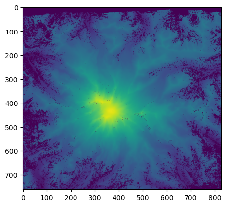
using plt.imshow(), we can visualize the array data contained in the raster dataset
[17]:
plt.imshow(array, vmin=500, vmax=4500);
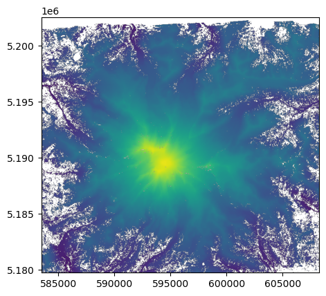
rasterio also offers rasterio.plot.show() to display rasters images and label the axes with geo-referenced extents. It also masks “nodata” cells.
[18]:
show(dataset, vmin=500, vmax=4500);
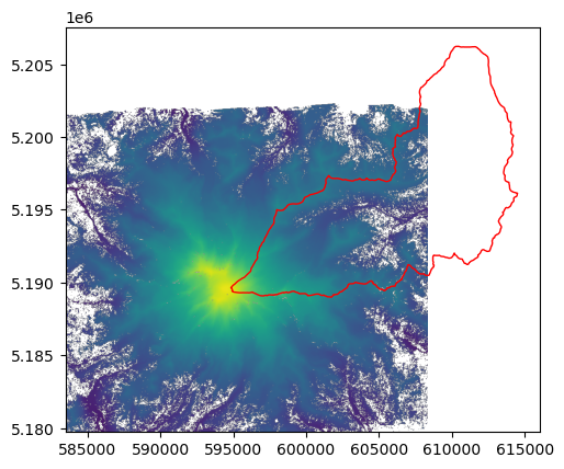
To plot a raster and a vector layers together, we need to initialize a plot object with plt.subplots, and pass the same ax argument to both plots. For example, let’s import the HUC12 polygon of the upper White River (see the GeoPandas notebooks for more information on working with geospatial vector data):
[19]:
import geopandas as gpd
white_riv_huc12 = gpd.read_file('data/rasterio/white_river_huc12.shp')
[20]:
fig, ax = plt.subplots()
show(dataset, ax=ax, vmin=500, vmax=4500)
white_riv_huc12.plot(ax=ax, edgecolor='red', facecolor='None');
Close the dataset when we’re done
the close() method is used to close a dataset, releasing the underlying file handle and any associated resources. This is important for proper resource management, especially when dealing with many files or in long-running processes.
[21]:
dataset.closed
[21]:
False
[22]:
dataset.close()
[23]:
dataset.closed
[23]:
True
Accessing and manipulating raster data
It is best practice to use rasterio.open() within a with statement. This ensures proper closing of the dataset and resource management, even if errors occur. You might recognize this syntax from working with files in notebook 04_files_and_strings.ipynb
[24]:
with rasterio.open(data_path / '20150818_rainier_summer-tile-30.tif') as dataset:
    array_m = dataset.read(1)
/tmp/ipykernel_7268/3173709603.py:2: DeprecationWarning: Setting the shape on a NumPy array has been deprecated in NumPy 2.5.
As an alternative, you can create a new view using np.reshape (with copy=False if needed).
  array_m = dataset.read(1)
[25]:
type(array_m)
[25]:
numpy.ndarray
Convert to units of feet
[26]:
array_ft = array_m * 3.2084
[27]:
plt.imshow(array_m,  vmin=500, vmax=4500)
plt.colorbar();
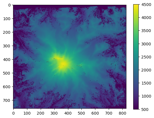
[28]:
plt.imshow(array_ft,  vmin=1600, vmax=14450)
plt.colorbar();
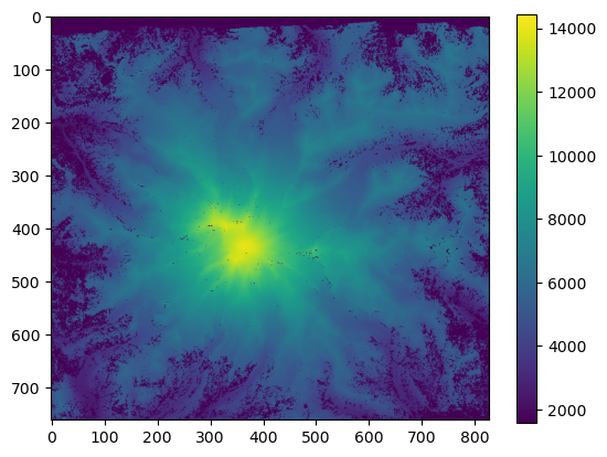
Looks the same! But notice the new units on the colobar scale.
Now let’s save this raster to a new file.
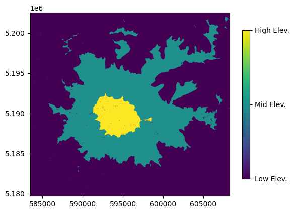
Make the data categorical
Bin the array data into three categories (1, 2, or 3) based on elevation values using numpy indexing
[29]:
array_classified = array_ft.copy()

array_classified[array_classified < 6000] = 1                                 # Low elevation zone, less than 6,000 ft
array_classified[(array_classified < 10000) & (array_classified > 6000)] = 2  # Mid elevation zone, between 6,000 and 10,000 ft
array_classified[array_classified >= 10000] = 3                               # High elevation zone, greater than 10,000 ft
[30]:
fig, ax = plt.subplots()

ct = show(array_classified, ax=ax, transform=dataset.transform)

im = ct.get_images()[0]
cbar = fig.colorbar(im, ticks=[1, 2, 3], shrink=0.8)
cbar.ax.set_yticklabels(['Low Elev. ', 'Mid Elev.', 'High Elev.']);
Writing Raster files
Writing a file with rasterio involves defining the characteristics of the output raster and then writing your data array to it.
The characteristics are provided in the form of metadata (or “profile”) which takes the form of a dictionary containing parameters we looked at above, including:
dimensions of the raster (height, width)
data type (dtype)
number of bands (count)
coordinate reference system (crs), and;
georeferencing transform (transform)
A word on transforms
In a raster dataset, an affine transformation is a mathematical mapping that relates the dataset’s internal pixel coordinates to a real-world coordinate system. This process, known as georeferencing, allows software to correctly display, scale, and align the image with other spatial data.
The affine matrix
A raster georeferencing transform can be expressed in mathematical terms using an affine matrix. This matrix defines a set of equations to convert a pixel’s row and column coordinates into real-world x-y coordinates.
Geospatial coordinate reference systems are typically defined on a cartesian plane with the 0,0 origin in the bottom left. Raster data uses a different referencing system. Rows and columns with the 0,0 origin in the upper left and rows increase and you move down while the columns increase as you go right.

Image from https://www.perrygeo.com/python-affine-transforms.html. More info on the Python Affine library.
[31]:
with rasterio.open(data_path / '20150818_rainier_summer-tile-30.tif') as dataset:
    transform = dataset.transform
    meta = dataset.meta

transform
[31]:
Affine(30.0, 0.0, 583464.253406,
       0.0, -30.0, 5202549.0989)
There are six elements in the affine transform (a, b, c, d, e, f)
a = width of a pixel
b = row rotation (typically zero)
c = x-coordinate of the upper-left corner of the upper-left pixel
d = column rotation (typically zero)
e = height of a pixel (typically negative)
f = y-coordinate of the of the upper-left corner of the upper-left pixel
rasterio provides an rasterio.Affine class, which can be used to create and manipulate new transforms
[32]:
transform = rasterio.Affine(
    a=30.0,
    b=0.0,
    c=583464.253406,
    d=0.0,
    e=-30.0,
    f=5202549.0989
)

transform
[32]:
Affine(30.0, 0.0, 583464.253406,
       0.0, -30.0, 5202549.0989)
… now back to writing that raster
[33]:
new_raster_file = data_path / '20150818_rainier_summer-tile-30_feet.tif'
The long way - specify metadata and close manually:
[34]:
out_dataset = rasterio.open(
    new_raster_file,
    mode='w',         # open file in write mode this time
    driver='GTiff',
    width=827,
    height=761,
    count=1,
    crs=32610,
    transform=transform,
    dtype='float32',
    nodata=0.0
)

out_dataset.write(array_ft, 1)
out_dataset.close()
The short way - use with and the original file metadata, meta, using ** to unpack the dictionary into arguments
[35]:
with rasterio.open(new_raster_file, 'w', **meta) as out_dataset:
    out_dataset.write(array_ft, 1)
Building a raster from scratch
Class activity
Create and write your own raster. This raster should be:
10 rows, 10 columns
The raster can contain any value(s) you want, but bonus points for a checkerboard pattern
Set upper left coordinates to:
xul: 569005.45
yul: 10746521.08
EPSG is 3070
Use the completed code blocks above as a template. Don’t be ashamed to adapt code you got from someone else or on the internet to accomplish something useful.
[ ]:
[ ]:
[ ]:
[ ]:
Masking (aka clipping) rasters using polygons
The rasterio mask function can be used to clip a raster to exclude areas outside of the polygon(s) defined in the shapefile.
[36]:
from rasterio.mask import mask
As an example, we can use the geometry information contained in the shapefile we plotted earlier as the mask
[37]:
white_riv_huc12.loc[0,'geometry']
[37]:

[38]:
crop_shape = white_riv_huc12['geometry']
A quick refersher - here’s what we’re working with:
[39]:
fig, ax = plt.subplots()
with rasterio.open(raster_file) as dataset:
    show(dataset, ax=ax, vmin=500, vmax=4500)
    white_riv_huc12.plot(ax=ax, edgecolor='red', facecolor='None');

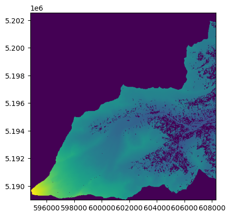
Now let’s use the mask function to clip the raster data with the polygon.
Set crop=True to crop the raster’s extent to the bounding box of the polygon(s).
[40]:
with rasterio.open(raster_file) as dataset:
    mask_image, mask_transform = mask(
        dataset,
        crop_shape,
        crop=True
    )
    mask_meta = dataset.meta

show(mask_image, transform=mask_transform);
[41]:
mask_meta.update({"driver": "GTiff",
                 "height": mask_image.shape[1],
                 "width": mask_image.shape[2],
                 "transform": mask_transform})

masked_file = data_path / '20150818_rainier_summer-tile-30_masked.tif'

with rasterio.open(masked_file, "w", **mask_meta) as out_dataset:
    out_dataset.write(mask_image)
[ ]: